

CHAPTER 4
THE EVOLUTION OF ALGEBRA, I
TRADITIONALLY, ALGEBRA WAS THE BRANCH of mathematics concerned with operations on—and equations involving—numbers. Taken in this sense, algebra is of great antiquity, since solutions to quadratic, cubic, and simultaneous equations are to be found inscribed on Babylonian stone tablets dating from 2000–1600 B.C.
Greek Algebra
The Greek mathematicians were primarily geometers, and it was accordingly natural that they should solve arithmetic and algebraic problems by means of geometric constructions, for example, by producing line segments whose lengths correspond to roots of equations. In this manner Euclid, for instance, solved problems equivalent to solving the systems of simultaneous equations xy = k2, x2 - y2 = a and xy = k2, x ± y = a.
The first substantial work in which arithmetic is treated in a manner wholly independent of geometry is the Introductio Arithmetica of Nicomachus of Gerasa (c. 100 A.D.). In this work, which is chiefly devoted to the arithmetic of the early Pythagoreans, numbers are used to denote quantities of objects—arithmoi—and not line segments as in Euclid. The work was extremely popular and actually used as a schoolbook down to the Renaissance.
Like all its predecessors, the Introductio is a rhetorical work in that no use of symbols is made, the exposition proceeding entirely verbally. The first work of algebra to employ symbols in any significant way—the first syncopated algebra (from Greek syncope, “cut short”)—was the Arithmetica of Diophantus, who flourished c.250 A.D. In this work Diophantus employs a character (probably the Greek letter ς, corresponding to our x) to represent the unknown quantity in an equation, and also uses initial letters to stand for equality and the operations of squaring and cubing.
The greater part of the Arithmetica is devoted to the solution of problems leading to linear and quadratic indeterminate equations, that is, equations without unique solutions. A few problems lead to equations of the third and fourth degrees. The general type of problem considered by Diophantus is to find two, three, or four numbers such that different expressions involving them in the first and second, and occasionally in the third degree, are squares, cubes, partly squares and partly cubes, etc.
53
54 |
CHAPTER 4 |
For example: To find three numbers such the product of any pair added to the sum of the pair yields a square; To find four numbers such that, if we take the square of the
sum ± any one of them singly, all the resulting numbers are squares; To find two numbers such that their product ± their sum gives a cube.
Diophantus recognized only positive rational solutions to these equations, and for this reason algebraic problems in which only rational (or integral) solutions are considered are today termed Diophantine.
Chinese Algebra
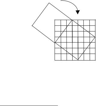
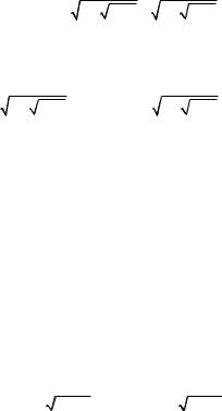
Algebra played a major role in early Chinese mathematics. While Chinese algebra was chiefly rhetorical, employing symbols only rarely (and then only in its later period), in contrast with Greek practice solutions to geometric problems were often cast in algebraic form. An arresting example of this occurs in the treatment of Pythagoras’s theorem to be found in the oldest of the Chinese mathematical classics, the Chou Pei Suan Ching—The Arithmetical Classic of the Gnomon and the Circular Paths of Heaven”—, which was probably composed during the Han period (206 B.C. – 222 A.D.). Here we see the square on the hypotenuse folded backwards1 onto the original
h |
a |
|
b |
triangle, manifestly containing three further identical triangles together with a square of side equal to the difference between the triangle’s base and altitude. An algebraic formulation is given rhetorically in the text, which, in modern terms may be written
h2 = 4ab/2 + (a – b)2 = a2 + b2,
1 It is possible that this demonstration was suggested by the Chinese art of paper-folding, since paper is believed to have been invented in China sometime before the first century B.C.

THE EVOLUTION OF ALGEBRA, I |
55 |
where h is the hypotenuse, a the altitude, and b the base. This demonstration is quite different from that of the Greeks.
The Chinese were adept at solving simultaneous linear equations, the coefficients of which they represented by means of rods on a counting-board, an arrangement precisely similar to that of numbers in a matrix (see below). The Chiu Chang Suan Shu—“Nine Chapters in the Mathematical Art”, c.100 B.C.—contains numerous problems requiring the solution of simultaneous linear equations of the type
ax + by = c a′x + b′y = c′.
Here the first equation was multiplied by a′ and the second by a, yielding, after subtraction,
y= ca '−c 'a ba '−b 'a
this result, as usual, being expressed in words.
In the Sun Tzu Suan Ching—“Master Sun’s Mathematical Manual”—of c.400 A.D. we find the following problem:
We have a number of things, but we do not know exactly how many. If we count them by threes we have two left over. If we count them by fives we have three left over. If we count them by sevens we have two left over. How many things are there?
This is a problem in number congruences, which, written in modern form, may be expressed as follows: determine a number N such that
N ≡ 2 (mod 3), ≡ 3 (mod 5), ≡ 2 (mod 7).
Sun Tzu gives 23 as a value for N, which is the least possible answer. This marks the beginnings of the famous Chinese Remainder Theorem of elementary number theory. The theorem states that, if we are given a set {m1, …, mk} of numbers no pair of which has a common factor apart from 1—such numbers are said to be relatively prime— then the system of congruences
x ≡ ai (mod mi), i = 1, 2, …, k,
has a unique solution modulo m1m2…mk .
By the fourteenth century the Chinese had developed the technique for generating approximate solutions to algebraic equations known in the West as Horner’s method (and published in 1819). For example, in the Ssu-Yuan Yü Chien—“Precious Mirror of the Four Elements”, which appeared in 1303—we find an approximate solution to the equation x3 – 574 = 0. First, noting that x = 8 is an approximate solution, y = x – 8 is substituted to yield the equation y3 + 24y2 + 192y – 62 = 0, which has a solution
56 |
CHAPTER 4 |
between 0 and 1. Taking y3 and y2 to be approximately 1 now gives y = 62(1+24+192) = 2 7 so that x = 58 7 .
In the “Precious Mirror” we also find a diagram of what is known in the West as Pascal’s triangle, which gives the coefficients of binomial expansions (a + b)n:
1
11
12 1
13 3 1
14 6 4 1
15 10 10 5 1 etc.
The author of the “Precious Mirror” refers to this diagram as “the old method for finding eighth and lower powers”, which shows that the binomial theorem must have already been understood by the Chinese at the latest by the start of the twelfth century.
Hindu Algebra
Significant contributions to algebra were also made by Hindu mathematicians during the period 200–1200 A.D. Hindu algebra was very close to being syncopated: to describe operations they used abbreviations of words together with a few special symbols, and for unknowns in equations they used the names of colours—black, blue, yellow, etc. The initial letter of each colour word was also used as a symbol. The Hindu mathematicians realized that quadratic equations had two roots, and they accepted the presence of both negative and irrational roots. They also took the important step of extending to irrational numbers the operations performed on integers, although this procedure lacked rigorous justification. For example Bhaskara shows how to add irrationals as follows. Given the irrationals √3 and √12, we get
√3 + √12 = √[(3 + 12) + 2√(3.12)] = √27 = 3√3. |
(*) |
Here Bhaskara is treating the irrationals as if they were integers, a fact he explicitly acknowledges. For if in the identity
m + n = √(m + n)2 = √(m2 + n2 + 2mn),
clearly true for integers m, n, we substitute √a for m and √b for n, we obtain
a + b = a + b + ab
of which (*) above is a special case.
The Hindus advanced well beyond Diophantus in their treatment of indeterminate equations, most of which derived from astronomical problems, their solutions
THE EVOLUTION OF ALGEBRA, I |
57 |
representing the appearance of certain constellations. Where Diophantus sought just a single rational solution to these equations, the Hindus developed methods for obtaining all integral solutions. Aryabhata devised a method—later employed by his successor Brahmagupta (fl. 628) for obtaining the integral solutions to the linear Diophantine
equation ax ± by = c, where a, b and c are positive integers. Let us outline this method,
using modern symbolism, in the case of ax + by = c.
First, we find the greatest common divisor (a, b) of a and b by means of the Euclidean algorithm. This involves performing the successive divisions:
a = bq1 + r1 b = r1q2 + r2 r1 = r2q3 + r3 r2 = r3q4 + r4
:
(0 < r1 |
< b) |
|
(0 < r2 |
< r1) |
|
(0 < r3 < r2) |
(1) |
|
(0 < r4 < r3) |
|
|
: |
|
|
so long as none of the remainders r1 > r2 > r3 > … |
are 0. After at most b steps the |
|
remainder 0 must appear: |
|
|
rn-–2 |
= rn–1qn+ rn |
|
rn–1 |
= rnqn+1 + 0 |
|
Now from the successive lines of (1) it |
follows that |
(a, b) = (b, r1) = (r1, r2) = … |
= (rn–1, rn) = (rn, 0) = rn. Therefore (a, b) is the last positive remainder in the sequence r1 > r2 > r3 > … . It also follows from (1) that if d = (a, b), then (positive or negative) integers k and A can be found such that
d = ka + Ab
(2)
For using the first equation in (1) we get
r1 = a – q1b,
so that r1 can be written in the form k1a + A1b . From the next equation, we obtain
r2 = b – q2r1 = b – q2(k1a + A1b ) = –q2 k1a + (1 – A1 )b = k2a + A2b .
This procedure can clearly be iterated through the successive remainders r3, r4, … until we arrive at a representation
rn = ka + Ab ,
as required.

58 |
CHAPTER 4 |
According to (2), our original equation ax + by = c has the particular solution x = k, y = A for the case c = d. In general, if c = d.q is any multiple of d, then from (2) we get
a(kq) + b( Aq ) = dq,
so that our original equation has the particular solution x = x* = kq, y = y* = lq. Conversely, if our equation has a solution x, y for a given c, then any solution must be a multiple of d = (a, b), for d divides a and b, and so must also divide c. Accordingly, we see that our equation has a solution if and only if c is a multiple of (a, b).
To determine the remaining solutions, we observe that if x = x′, y = y′ is any solution other than the one x = x*, y = y* just found by the use of the Euclidean algorithm, then x = x′ – x*, y = y′ – y* is easily seen to be a solution to the equation
ax + by = 0. |
(3) |
Now the most general solution to (3) is
x = rb/(a, b), y = –ra/(a, b).
For, dividing (3) by (a, b) = d, we obtain
a′x + b′y = 0,
where a′ = a/d and b′ = b/d are relatively prime. Therefore
a′x = –b′y |
(4) |
and since b′ is relatively prime to a′, it must divide x, i.e., x = rb′ for some integer r. From (4) it now follows that y = –ra′, as claimed.
Accordingly the general solution to our original equation, assuming c to be a multiple of (a, b) is
x = x* + rb/(a, b), y = y* – ra/(a, b).
This is essentially Brahmagupta’s solution.
Brahmagupta also considered the Diophantine quadratic equation2 x2 = 1 + py2. Later the medieval mathematician Bhaskara, in a remarkably impressive feat of calculation, furnished particular solutions to this equation for p = 8, 11, 32, 61 and 67.
2 This equation was mistakenly named for the English mathematician John Pell (1611–1685), but was actually first considered by Archimedes.
THE EVOLUTION OF ALGEBRA, I |
59 |
Arabic Algebra
Algebra entered Arabic (or Moslem) culture through the medium of a treatise on equations—based in the main on the work of Brahmagupta, but also showing traces of Greek and Babylonian influence—written in 830 by the mathematician Mohammed ibn Musa al-Khwarizmi. It is from the title of this treatise, Al-jabr w’al muqâbala, which in free translation means “Restoring and simplification”, that the word “algebra” originates3. Here the word “al-jabr” meant restoring the balance of an equation by adding or subtracting on one side a term which had been removed from the other, as in transforming x2 + 4 = 6 into x2 = 6 – 4 = 2. The word “al-muqâbala” meant simplification of an equation in the sense of subtracting equal terms from both of its
sides or combining several similar terms into a single term, for example 2x2 and 4x2 into 6x2.
The algebra of al-Khwarizmi holds a most important position in the history of mathematics, since the subsequent Arabic and medieval works on algebra were founded on it, and, moreover, it served as the conduit through which the Hindu-Arabic system of decimal notation was introduced into the West. However, in certain respects al-Khwarizmi’s work is a backward step from that of Brahmagupta, and even from that of Diophantus. The problems treated are far more elementary than those discussed by the latter, and in particular there is little discussion of indeterminate equations. Also alKhwarizmi’s algebra is entirely rhetorical. Nevertheless, the straightforward character and clear argumentation of the work makes it very much a forerunner of today’s school algebra texts.
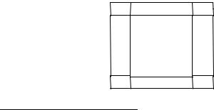
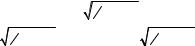
In his algebra al-Khwarizmi solves linear and quadratic equations by “completing the square” and recognizes that the latter can have two roots4—but at the same time he rejects negative roots. He also solves a number of quadratic equations by means of geometric arguments. For instance, to solve the equation x2 + 10x = 39 he draws a
square ab to represent x2, and on |
the four |
sides of this square he places |
rectangles c, d, e, and f, each 22 units |
wide. To |
complete the larger square, the |
c
a
f |
d |
b
e
3It is of interest to note that the word “algorithm” derives from the author's name. Curiously, “al-jabr” also came to mean “bonesetter” and in sixteenth century Italy the word “algebra” meant the art of restoring or setting broken bones.
4 The term “root” as a solution to an equation originates with al-Khwarizmi’s use of the same word —in its botanical sense— for the unknown in an equation.

60 |
CHAPTER 4 |
four small corner squares, each having an area of 6 14 units, are added. Thus to “complete the square” one adds 4 × 6 14 = 25 units, so obtaining a square of total area 39 + 25 = 64 units. The side of the larger square must accordingly be 8 units, from which we subtract 2 × 2½ = 5 units, to find that x = 3.
Other significant algebraists of the Moslem world include Abu’l-Wefa (940–988), al–Karkhi (c.1029) and the Persian Omar Khayyam (c.1100), known to posterity as the author of the enchanting Rubaiyat. Abul-Wefa gave geometric solutions to some specific quartic equations, and it is believed that al-Karkhi provided the first numerical solutions to such equations as ax2n + bxn = c, in which the Diophantine restriction to rational solutions has been relaxed. In doing so al-Karkhi took the first significant step towards the solution by radicals of algebraic equations of higher than second degree which was to prove of such importance in the later development of algebra.
Omar Khayyam—who regarded algebra as “proven geometric facts”—devoted most of his mathematical efforts to the solution of cubic equations. However, he provided only geometric solutions, mistakenly believing that arithmetic solutions to such equations were, in general, impossible. But he took the significant step of using intersecting conics to solve the general cubic equation (with positive roots), thereby extending the work of Menaechmus and Archimedes. He observes that, since it contains a cube, this equation cannot be solved by plane geometry, that is, by the use of straightedge and comapasses alone. Hampered by the purely rhetorical nature of his algebra, Omar Khayyam had to resort to circumlocutions of painful tortuosity to express his ideas—a far cry from the elegant quatrains of the Rubaiyat. In modern notation, his method of solving the cubic went like this. Given a cubic x3 + ax2 + bx + c = 0, substitute 2py for x2, to obtain 2pxy + 2apy + bx + c = 0. The latter is the equation of a hyperbola, and the equation x2 = 2py that of a parabola. The abscissas of the points of intersection of the two curves will be the roots of the given cubic equation.
Algebra in Europe
The first algebraic work of significance to appear in medieval Europe was the Liber Abaci (1202) of Leonardo of Pisa (c.1175–1230), also known as Fibonacci. The work’s title, which means “Book of the Abacus”, is highly misleading, since the use of the abacus is not discussed at all. On the contrary, in it the use of Hindu-Arabic numerals is strongly advocated. It is in the Liber Abaci that we first encounter the celebrated Fibonacci sequence 1, 1, 2, 3, 5, 8, 13, 21, …, in which each term after the second is the sum of its two immediate predecessors. Amusingly, this sequence arises as the solution to a problem involving the breeding of rabbits! The sequence has been shown to have many interesting properties, for example, successive terms are relatively prime, and the nth term5 is given by the expression
5 I owe to Gerard Khatcherian the observation that the nth term of the Fibonacci sequence may be identified as the total number of ways of ascending an n-stepped staircase taking one or two steps at a time.
THE EVOLUTION OF ALGEBRA, I |
61 |
(1 + 5)n − (1 − 5)n . 2n 5
In the Liber Abaci and in two later works, the Liber Quadratorum and the Flos (both 1225), Fibonacci describes, in rhetorical form, solutions of determinate and indeterminate equations of the first and second degree, as well as some cubic equations. Most remarkable is his discussion of the cubic equation x3 + 2x2 + 10x = 20. He proves that this equation cannot have a “Euclidean” root of the form a +√b with rational a and b. He then states an approximate answer which, expressed in decimal notation, is correct to nine places. This is the most accurate approximation to an irrational root given in Europe up to that time, and exactly how it was obtained remains a mystery to this day. The Liber Quadratorum contains solutions to a variety of problems in indeterminate analysis: for example, in find a rational number x such that both x2 – 5 and x2 + 5 are squares of rational numbers, Fibonacci obtains the correct solution 4112 .
Fibonacci makes frequent use of the identity
(a2 + b2)(c2 + d2) = (ac + bd)2 + (bc – ad)2 = (ad + bc)2 + (ac – bd)2,
which had appeared in Diophantus and was also known to the Arabs.
A figure of pivotal importance in the development of algebra was the Frenchman François Viète (1540–1603). He was probably the first to conceive of algebra in something close to its modern sense as being equally applicable to geometric magnitudes and numbers. For Viète, algebra was a general method of reasoning about “species” or forms of things—for this reason he calls algebra logistica species in his Isagoge in Artem Analyticam (“Introduction to the Analytic Art”) of 1591. In this work, the first genuinely (even if not fully) symbolic algebra, Viète makes a clear-cut distinction between the idea of a parameter (e.g., a coefficient in an equation) and that of unknown quantity, using consonants to stand for the former and vowels the latter. Viète saw clearly that in studying the general quadratic equation ax2 + bx + c = 0 (in modern notation), one was actually studying an entire class of equations. Viète was also possibly the first to note some of the relations between the roots and coefficients of an equation: for instance, the fact that if the cubic equation x3 + b = 3ax has two positive roots u and v, then 3a = u2 + uv + v2 and b = uv2 + vu2.
The Solution of the General Equations of Degrees 3 and 4
A major influence on the development of algebra has been the attempt to formulate general schemes of solutions for equations. While the method for solving quadratic equations of “completing the square” was in essence known to the ancient Babylonians, general solutions to cubic and quartic equations did not appear until the sixteenth century in Italy. The general solution to the cubic equation x3 + ax2 + bx + c = 0 was first discovered around 1500 by Scipione del Ferro (1465–1526), and apparently independently in 1530 by Nicolò Tartaglia (1499–1557). Tartaglia’s solution was
62 |
CHAPTER 4 |
actually published by Girolamo Cardano (1501–1576) in his Ars Magna of 1545 and for this reason is known as Cardano's solution (although Cardano, it is true, does credit Tartaglia with the solution).
The Ars Magna is largely rhetorical but in modern notation the method of solving the cubic presented in it may be briefly presented as follows. We first remove the quadratic term ax2 by putting x = y – 13 a: this changes the equation into the form
y3 + py + q = 0, where the coefficients p, q are readily expressible in terms of the original coefficients a, b, c. If we now write y = u + v, then the equation becomes
u3 + v3 + (3uv + p)y + q = 0.
Thus, if we choose u and v to to satisfy
3uv + p = 0,
we obtain the two simultaneous equations
13 u3 + v3 = –q u3v3 = –p3/27
for the two unknowns u3 and v3. By eliminating one of these, we find that the other satisfies the quadratic equation
t2 + qt – p3/27 = 0.
The two roots of this equation are u3, v3 and so, using the quadratic formula to write down these roots, we obtain
u3 = −q 2 + q2 4 + p3 27 |
v3 = −q 2 − q2 4 + p3 27 |
whence finally
y = u +v = 3 −q 2 + q2
  4 + p3
  27 + 3 −q
 2 − q2
  4 + p3
  27
27
An expression involving only the arithmetic operations and the extraction of roots—such as that on the right side of the equation immediately above—is called a radical. For this reason it is said that Cardano’s procedure shows that the general cubic equation is soluble by radicals.
As Cardano recognized, this method of solution leads to trouble in the socalled irreducible case when the equation has three real roots (the only other possible number of real roots being 1). To see what happens, consider as an example the equation x3 –2x2 – x + 2 = 0. The left hand side factorizes as (x + 1)(x –1)(x –2), so the equation has as three real roots –1, 1, 2. Performing the required calculations in Cardano's procedure, we find that p = −7 3 , q = 20 27 , so that q2/4 + p3/27 = −972542 = −13 . But now Cardano's formula tells us to take the square root of this number, which
is negative! Thus, although the roots of the original equation are known to be real,

THE EVOLUTION OF ALGEBRA, I |
63 |
Cardano's method will not furnish the solution unless one is prepared to countenance the use of complex numbers. In fact the formula gives (recalling that we write i = √–1)
y = u +v = 3 −10 27 + 13 i + 3 −10 27 − 13 i
This expression gives a real result because, while the cube roots in it are all individually complex, their sum turns out to be real and gives the correct value for6 y.
It is worth noting in this connection that in 1591 Viète formulated a solution to the cubic in which use is made of a trigonometric identity involving the cosine function cos A of an angle A, so bypassing Cardano’s formula, and avoiding altogether the use of complex numbers in the irreducible case. He starts with the well-known identity expressing the cosine of 3A in terms of the cosine of A:
cos 3A = 4cos3A – 3cos A, |
|
and writes z = cos A to obtain |
|
z3 – ¾ z – 14 cos 3A = 0. |
(1) |
If the given cubic is |
|
y3 + py + q = 0, |
(2) |
then by substituting y = hz and choosing h appropriately the coefficients of (2) can be made to coincide with those of (1). Making this substitution in (2) gives
z3 + (p/h2)z + q/h3 = 0. |
(3) |
We require that p/h2 = –¾ so that h = √– 4 3 p. Now we select an angle A to satisfy
q/h3 = – 14 cos 3A,
that is, to satisfy
cos 3A = –4q/h3 = −q 2 − p3 27 = k. |
(4) |
If the three roots of (3) are real then it can be shown that p is negative—so that h is real— and also that |k| < 1, so that an angle A can be chosen to satisfy (4). In that case z = cos A satisfies (1), hence also (3), and so y = z/h satisfies (2).
6Actually there are three pairs of values for u and v, namely |
(–5 + i√3)/6, |
(–5 – i√3)/6; |
(1 – 3i√3)/6, |
(1 + 3i√3)/6; and (4 + 2i√3)/6, (4 – 2√3i)/6. Summing each |
pair gives y = |
−5 3 or 13 or |
13 , whence |
x = y + 23 = –1 or 1 or 2. |
|
|
|
64 |
CHAPTER 4 |
Viète obtained only the single root z = cos A but in fact the remaining roots are easily obtained. For observe that, if A is any angle satisfying (4), then z = cos A satisfies (3). But clearly, if A satisfies (4), then so do A + 120° and A + 240°. It follows that z = cos(A + 120°) and z = cos(A + 240°) are the remaining roots.
It is striking that the first genuine use of imaginary or complex numbers was made in the theory of cubic equations, and not, as might be supposed, in the theory of quadratic equations, where they are customarily introduced nowadays. In the case of cubic equations it was clear that real solutions actually existed, even if presented in a bizarre form, so that the appearance of imaginary quantities could not be avoided, as in the case of quadratic equations, by the mere claim that the equation had no solutions. This was the first step in the process which culminated in the nineteenth century with the complete acceptance of complex numbers
While—as we have seen—Cardano’s formula suggests that the sum of complex radicals can give a real result, Cardano himself seems to have remained mystified by the apparent fact and never fully accepted it. The genuineness of the phenomenon was first recognized by Cardano’s disciple Rafaello Bombelli (c.1526–1573). In Bombelli’s L’Algebra of 1579 he observes that Cardano’s formula applied to the irreducible equation x3 – 15x = 4 yields the solution
x = 3 2 + −121 + 3 2 − −121
while direct substitution shows that x = 4 is the sole positive solution. It occurred to him that these apparently conflicting facts could be reconciled if it were the case that
3 2 + −121 = 2 + √–1, 3 2 − −121 = 2 – √–1 |
(5) |
To this end Bombelli lays down rules for the manipulation of imaginary numbers which are strikingly close to those found in modern expositions. He represents complex numbers as “combinations” of four basis elements, which he terms piu “more” (+1), meno “less” (–1), piu di meno “more than less” (+√–1), meno di meno “less than less” (–√–1). Using his rules, Bombelli proceeds to establish the relations (5): in modern notation, the first of these is verified as follows:
(2 + i)3 = 8 + 3.4i + 3.2.i2 + i3 = 8 + 12i – 6 – i = 2 + 11i.
Unfortunately, Bombelli’s ingenious maneuver was of no help in actually producing numerical solutions of irreducible equations, for any attempt to determine algebraically the cube roots of the complex numbers in Cardano’s formula invariably leads back to the very cubic whose solution was sought in the first place. For instance, if one tries to determine real a and b so that
a + bi = 3 2 +11i , a – bi = 3 2 −11i |
(6) |
then

THE EVOLUTION OF ALGEBRA, I |
65 |
(a + bi)3 = 2 + 11i. |
|
Expanding the left side and equating real parts gives |
|
a3 – 3ab2 = 2. |
(7) |
But if we multiply the two equations in (6) together, we find
a2 + b2 = (a + bi)(a – bi) = 3 4 +121 = 5, so that b2 = 5 – a2. Substituting this value for b2 into (7) then gives
4a3 – 15a = 2. Setting x = 2a in this yields the equation
x3 – 15x = 4,
precisely the equation we started with. This fact justifies the use of the term “irreducible”.
After the solving of the general cubic equation it was natural to try to deal similarly with equations of degree 4 (quartic or biquadratic equations). The general solution to these was discovered by Cardano’s pupil Ludovico Ferrari (1522–1565), and also appears in the Ars Magna, where Cardano writes that the method is “due to Luigi Ferrari, who invented it at my request.” The method involves reducing the problem to the solution of cubic and quadratic equations. Here, in modern notation, is one version of it.
Consider the equation
x4 + ax3 + bx2 + cx + d = 0.
To both sides add (ex + f)2, so obtaining |
|
x4 + ax3 + (b + e2)x2 + (c + 2ef) x + (d + f2) = (ex + f)2. |
(8) |
Now choose e and f so as to make the left side a perfect square of |
the form |
(x2 + px + q)2. Expanding this and comparing coefficients of powers of x, we obtain 2p = a, p2 + 2q = b + e2, 2pq = c + 2ef, q2 = d + f 2.
This fixes the value of p. The remaining equations may be written in the form e2 = p2 + 2q – b, 4e2f2 = (2pq – c)2, f 2 = q2 – d.
If we substitute the first and third of these into the second, we get
66 |
CHAPTER 4 |
(2pq – c)2 = 4(p2 + 2q – b)( q2 – d),
that is, using p = ½a,
(aq – c)2 = (a2 + 8q – 4b)(q2 – d).
This is a cubic equation in q and so can be solved for q in terms of a, b, c, d. Once a root has been obtained, the equations above yield the values of e and f. Equation (8) then becomes
(x2 + px + q)2 = (ex + f)2,
that is,
[x2 + (p + e)x + (q + f)] [x2 + (p – e)x + (q – f)] = 0.
Thus we finally get two quadratic equations |
|
x2 + (p + e)x + (q + f) = 0, |
x2 + (p – e)x + (q – f) = 0, |
whose roots are the four roots of the original equation.
The significance of the discovery of general methods of solving these equations lies not in the details of the procedures themselves, but rather in the fact that these methods show that the roots of any polynomial equation of degree up to 4 can be expressed in terms of the coefficients of the equation using only the operations defined in the field of complex numbers, together with the extraction of roots. This fact, accordingly, was in essence known before 1600.
The Algebraic Insolubility of the General Equation of Degree Greater than Four
In developing methods for solving polynomial equations it was natural that attention should come to be directed to the question of exactly how many roots an equation possessed. Both Cardano and Descartes asserted that a polynomial equation of degree n has exactly n (real or complex) roots, but gave no proof. In the eighteenth century Euler, D’Alembert and Lagrange each formulated a putative proof, but none of them showed that a root actually existed in the first place. This latter fact—the Fundamental Theorem of Algebra—was first given a solid proof by Gauss in 1799. At the same time Gauss showed that an nth degree polynomial can be expressed as a product of linear and quadratic factors with real coefficients—a fact which had been recognized, but not rigorously proved, by his predecessors. An important feature of Gauss’s work is that, while it establishes the existence of a root, it provides no means of actually calculating it. This is probably the first example of a pure existence proof in mathematics.
Although prior to Gauss’s rigorous proof of the fact it was morally certain that all polynomial equations with real coefficients possessed roots, attempts to obtain roots of equations of degree higher than 4 by algebraic means had met with persistent failure. In

THE EVOLUTION OF ALGEBRA, I |
67 |
1770 the great French mathematician Joseph-Louis Lagrange (1736–1813) undertook a systematic analysis of the methods of solving third and fourth degree equations in the hope that an understanding of exactly why these methods worked might furnish a clue as to how to solve higher degree equations. Lagrange observed that to solve an equation of degree n = 3 or 4 one introduces a certain rational function7 f—a resolvent function—of the roots of the equation which is then shown itself to satisfy an equation of lower degree than that of the original; this latter equation—the reduced equation— can be solved algebraically and its roots then yield a solution to the given equation. To explain why the reduced equation is of lower degree, Lagrange proved the general result that if a rational function f of the roots of a polynomial equation assumes exactly r values when the roots of the equation are permuted arbitrarily, then f itself is a root of an equation of degree r whose coefficients are rational functions of the coefficients of the given equation. In the cases n = 3 and 4 the function f can be chosen to assume exactly n – 1 different values under arbitrary permutations of the roots of the given equation, so in both cases the reduced equation is of lower degree.
Lagrange sought to extend this technique to the general quintic (degree 5) equation, and so sought a resolvent function for this case which would satisfy an equation of degree less than 5. But his efforts were in vain, which led him to suspect that the solution of the general equation of degree higher than 4 was impossible.
While Lagrange failed to resolve the problem of the algebraic solubility of general higher-degree equations, his analysis of the problem provided the basis for the work of his successors Abel and Galois, who were finally to establish the algebraic insolubility of the general equation of degree > 4. Moreover, Lagrange’s insight that one should consider the values that a rational function assumes when its variables are permuted led to the theory of permutation groups (see below).
Lagrange’s work on equations had a direct influence on the Italian mathematician Paolo Ruffini (1765–1822), who during the first decade of the nineteenth century made several inconclusive attempts to prove that the general equation of degree > 4 did not admit of algebraic solution. Ruffini did succeed in establishing that no rational function of the n roots of an equation of degree n > 4 exists which assumes just 3 or 4 values, so proving that no resolvent function in Lagrange’s sense could be found which satisfies an equation of degree < 5.
In 1801 Gauss made an important contribution by showing that every binomial equation—that is, of the form xn – a = 0—is algebraically soluble (the cyclotomic equation is the case a = 1). Nevertheless, he regarded this as a special case, sharing with Lagrange the suspicion that the general equation would prove to be algebraically insoluble.
The problem was finally settled by the Norwegian mathematician Niels Henrik Abel (1802–29). While still at school he had read Lagrange’s and Gauss’s—but not, it seems, Ruffini’s—work on the theory of equations and at first believed that Gauss’s solution of binomial equations could be extended to the general quintic. Soon realizing his error, he then tried to prove that the quintic was algebraically insoluble, an effort which in 1826 was to be crowned with success. It is remarkable that he succeeded in doing this by proving—apparently in total ignorance of Ruffini’s work—a result which
7 A function is said to be rational if it is the quotient of two polynomials.

68 |
CHAPTER 4 |
the latter had assumed without proof, namely, that the roots of an algebraically soluble equation can always be cast in such a form that each of the radicals in them is a rational function of the roots of the equation together with the roots of unity. The insolubility of the general quintic equation is known today as the Ruffini-Abel Theorem.
In his work Abel also discovered a general class of algebraically soluble equations. These, the Abelian equations, are those with the property that all their roots are rational functions of any one of them. More precisely, an equation is Abelian if, given any root a, there are rational functions θ1, …, θn–1 such that the roots of the equation are given
by a, θ1(a),…, θn–1(a) and, in addition, the θi commute on a in the sense that θi(θj(a)) = θj(θi(a)). The cyclotomic equation xn – 1 = 0 is Abelian in this sense, since, as we have seen on p.40, its roots are representable as powers of any one of them. Other important concepts introduced by Abel are those of a field of numbers and of a polynomial irreducible over a given field. A polynomial is said to be reducible over a given field if it can be expressed as the product of two polynomials of lower degree with coefficients in the field; in the opposite case it is irreducible. For example, x2 + 1
is irreducible over the real field \, but x2 – 1 is reducible, as it can be expressed as the
product (x + 1)(x – 1).
Abel’s work had left open the question of exactly which equations are, or are not, soluble. This and other questions were answered by Évariste Galois (1811–32), whose work—the revolutionary significance of which went quite unrecognized by his contemporaries—proved to be instrumental in laying the foundations for what was later to become known as abstract algebra.
In his analysis of algebraic equations Galois took from Lagrange the idea of a permutation of the set of roots of an equation. Here we may consider a permutation to be any change in the ordered arrangement of a set of objects (or symbols). For example, the permutation in which the order of the letters a, b, c is changed to c, a, b is written (acb), the notation indicating that each letter is taken into the one immediately following, the first letter being understood to be the successor of the last. Thus in the permutation (acb), the letter a goes to c, c in turn to b and finally b to a. The notation (ac), in which b is omitted, signifies the permutation in which a goes to c, c to a and b remains fixed. If two permutations are performed successively, the resulting permutation is called the product or composite of the two permutations. Thus the product of (acb) and (ac), written (acb)(ac), is the permutation (bc). Notice that the operation of forming the product of permutations is not commutative, that is, it depends on the order in which the permutations are performed. Thus, for example, (ac)(acb) = (ab), while we have seen that (acb)(ac) = (bc). The permutation I which leaves all letters fixed is called the identity permutation: clearly the product of I with any permutation leaves the latter unchanged. Notice also that, for any permutation P there is a unique inverse permutation whose product with P in either order is the identity permutation I. Thus, for example, since (acb)(bca) = (bca)(acb) = I, the inverse of (acb) is (bca). We may sum this up by saying that the collection of all 6 permutations on the set {a, b, c}, together with its product operation, forms a group8, called the permutation group on 3 elements. Similarly, the collection of n! = 1.2.3....n permutations of n distinct objects—written Sn—forms the full permutation group on n
8 The group concept will be formally introduced later in the section on abstract algebra.
THE EVOLUTION OF ALGEBRA, I |
69 |
elements. By a subgroup of a group we mean a part of it which contains the product and inverse of any of its elements. (Thus the three permutations (abc), (abc)2 and (abc)3 = I form a subgroup of the full permutation group S3 on 3 elements.) A subgroup of the full permutation group on n elements will simply be called a group of permutations on n elements.
The problem of solving a polynomial equation by radicals was, as Galois grasped, essentially that of finding radicals whose introduction will make the given equation reducible. For example, the general quadratic equation x2 + px + q = 0 is not reducible
but it becomes so on introducing the radical 14 p2 −q , for then x2 + px + q becomes
factorizable as [x + 2p + 14 p2 −q ][x + 2p – 14 p2 −q ]. Galois associated
with each polynomial equation a certain group of permutations of its roots—its Galois group—whose properties as a group reflect faithfully the properties of the equation. He showed that, in the case of an equation soluble by radicals, each time an appropriate radical is introduced the associated group of permutations is diminished in such a way as to become a certain kind of subgroup of its predecessor. When all the radicals necessary for solving the equation have been introduced—and the polynomial reduced to a product of linear factors in these radicals—the associated group is reduced to the subgroup consisting of just the identity element. In this way the algebraic solubility, or solution by radicals, of the equation is found to correspond to the existence of a sequence of subgroups of its Galois group satisfying a certain condition (somewhat too involved to be formally introduced here), in which case the Galois group is said to be solvable. The algebraic solubility of the equation is thus transformed into the solvability of its Galois group. In the case of the general quintic equation, the Galois group is the full permutation group S5 on 5 elements, which is not solvable. It follows that the general quintic equation is not algebraically soluble. Certain specific equations, for instance x5 – x – 1 = 0, can also be shown to have S5 as their Galois group, so they are not algebraically soluble either. On the other hand, since all permutation groups on 2, 3, or 4 elements are solvable, all equations of degrees 2, 3, or 4 are algebraically soluble, as we already know. The Galois group of each of the algebraically soluble equations studied by Abel has the property that products within it are commutative (and so solvable), that is, for any permutations P, Q,
PQ = QP.
A group satisfying this condition is for this reason called Abelian.
Galois theory (as it is known) thus provides a complete analysis of the solubility of polynomial equations. It can also be used to demonstrate the impossibility of trisecting a general angle, or of doubling the volume of a cube, by ruler and compass constructions. Given a geometric construction problem, one first sets up an algebraic equation whose solution is the desired quantity: for example, in the case of doubling the cube, the equation is x3 – 2 = 0. The condition for solubility of the construction problem with Euclidean tools is that the equation be algebraically soluble by the successive extraction of square roots. In terms of Galois theory a necessary and sufficient condition is that the number of elements of the Galois group of the equation be a power of 2. This can be shown not to be the case for the equations corresponding

70 |
CHAPTER 4 |
to the doubling of the cube and the trisection of the angle, so neither of these problems is soluble by means of Euclidean tools9 (see Appendix 1 for an elementary proof of these facts).
Early Abstract Algebra
Although the group concept is chronologically the first of those we now classify as falling under “abstract algebra”, it did not in fact play an explicit role in the early development of the subject, which took place in England and Ireland during the first half of the nineteenth century. The central idea of the algebraists of the “British school”—which included Sir William Rowan Hamilton (1805–1865), Augustus de Morgan (1806–1871), and George Boole (1815–1864)—was to investigate the algebraic laws holding of the various number systems, and of mathematical systems in general, in a purely symbolic manner. In de Morgan's symbolic algebra, for example, letters A, B, C and symbols of operation + and – are understood as being of an entirely abstract character, and so not necessarily signifying numbers or magnitudes and operations thereupon. Indeed de Morgan claims that “with one exception [that of the equality symbol], no word or sign of arithmetic has one atom of meaning..., the object of which is symbols and their laws of combination, giving a symbolic algebra which may hereafter become the grammar of a hundred distinct significant algebras.”
Despite de Morgan’s insistence on the arbitrary nature of the signs of his algebra, he seems not to have appreciated that this arbitrariness should also be extended to their laws of combination. He was still sufficiently influenced by Kantian philosophy to believe that the basic laws of the algebra of number systems—commutativity, associativity and the like—would apply to any algebraic system whatever. He was proved wrong in this by Hamilton’s later invention of the algebra of quaternions (see below).
Important contributions to the development of abstract algebra were made by Boole in his two works, The Mathematical Analysis of Logic (1847) and An Investigation of the Laws of Thought (1854). Boole’s system—known nowadays as Boolean algebra— as presented in these two works embodies the first successful application of algebraic methods to logic.
Boole seems to have had several interpretations of his algebraic system in mind. In his 1847 work he thinks of each of the basic symbols of his “algebra” as standing for the mental operation of selecting just the objects possessing some given attribute or included in some given class. In 1854 he conceives of these symbols as standing for the attributes or classes themselves. He also recognizes that the algebraic laws he proposes are satisfied if the basic symbols are interpreted as taking just the number values 0 and 1, yielding a system of binary arithmetic.
Boole used letters x, y, z,... to represent sets of things—numbers, points, lines, ideas, or other entities—selected from a universal set or universe of discourse which he denoted by the number 1. For example, if the symbol 1 designates the class of all
9 It should be pointed out that these two problems, which had plagued mathematicians since antiquity, had been quietly settled in the negative in 1837, before the application of Galois theory, by the French mathematician Pierre Wantzel (1814–1848).
THE EVOLUTION OF ALGEBRA, I |
71 |
Canadians, then x might stand for the subclass consisting of all Canadians under twenty-one and y for the subclass of Canadians over six feet tall. The number 0 Boole took to designate the empty class, that is, the subclass of the domain of discourse having no members. The addition symbol + was taken by Boole to signify disjoint union, so that x + y denotes the class of all objects that are either in x or in y, but not in both. The multiplication symbol . was understood to mean intersection, so that x.y (or xy) denoted the class of all objects in both x and y. The sign = was, as usual, taken to indicate identity. The resulting “Boolean” algebra is then a field in which not all of the rules of ordinary algebra hold: for example, in it 1 + 1 = 0, x.x = x and x(1 – x) = 0 for arbitrary x.
Boole showed that his algebra provided a simple and effective means of presenting syllogistic reasoning. The equation xy = x, for example, expresses the assertion that all x’s are y’s. If now in addition yz = y, i.e. if all y’s are z’s, then we get
xz = (xy)z = x(yz) = xy = x,
i.e. all x’s are z’s.
Boole’s ideas have since undergone extensive development, and the concept of Boolean algebra now plays a central role in mathematical logic and the design of computer circuits.