

Asperti A.Categories,types,and structures.1991
.pdf
|
5. Universal Arrows and Adjunctions |
the rules |
are interpreted by the fact that |
(weakenings) |
each morphism f: 1→∆ |
|
gives a morphism f˚εa: !a→∆ |
(contractions) |
each morphism f: !a!a→∆ |
|
gives a morphism f˚δa: !a→∆ |
(!,l) |
each morphism f: a→∆ |
|
gives a morphism f˚Ea: !a→∆ |
(!,r) |
each morphism f: !c→a |
|
gives a morphism !f˚Dc: !c→!a . |
As for the rules which contain ?, their meaning is easily derivable by duality. The idea is to define a functor ? : C→C by
? = * ˚ ! ˚ *
that is ?A = (!A*)*. Then the following theorem gives the categorical meaning of the modality ?, why not.
5.5.6 Theorem Let <C,(!,D,E)> be an !-model. Then there exist a monad (?, D': ?˚ ?→?, E': Id→?) and natural isomorphisms
|
I': ?(A B) ?(A) ?(B) |
|
|
|
|
J': ?0 , |
|
|
|
where 0 |
and are the identities for and , |
the duals of the Cartesian and tensor products in |
||
C . |
|
|
|
|
Proof. Set ? = * ˚ ! ˚ * : C → C and, for each object A, D'A = (DA*)* |
and E'A = (EA*)*. As |
|||
D: !→!°!, |
one has |
|
|
|
|
DA*: !A*→!°!A* |
|
|
|
|
(DA*)*: (!°!A*)*→(!A*)* |
|
by def.of |
(-)* |
|
(DA*)*: (!°*°*°!A*)*→(!A*)* |
by Id (-)** |
||
|
D'A: ?°?A→?A |
|
|
|
Each of these steps is an isomorphism, uniform in |
A, and gives a natural transformation D': ?˚?→?. |
|||
Similarly, from Ε: !→IdC one has EA*: !A*→A* |
and, thus, E'A = (EA*)*: A→?A. The |
|||
properties required for a monad follow by duality. |
|
|
|
|
As for the natural isomorphisms, compute |
|
|
|
|
|
?(A B) = * ˚ ! ˚ *(A B) |
|
|
|
|
= * ˚ !(A*∩B*) |
|
by theorem 4.4.6 |
|
114
5. Universal Arrows and Adjunctions
(!(A*) !(B*))* |
by def. of !-model |
= ?A ?B |
by theorem 4.4.6. |
Finally, ?0 = * ˚ ! ˚ *0 * ˚ ! t 1* , |
by definition and theorem 4.4.6. ♦ |
Exercise Endow a structure of monoid over each object in a monoidal category whose tensor product is actually a Cartesian coproduct. Then give the details of the interpretation of the rules for ?.
Next we find, within any categorical model of linear logic, an interpretation for the intuitionistic connectives ∩ and , by using the comonad construction in the !-model. Namely, given an !- model C, one may interpret intuitionistic “and” and “implication” by Cartesian product and exponential in a suitable category derived from C. As the purpose of the iterator ! was to take us back to intuitionistic logic, we use its categorical meaning to construct this new category.
As a matter of fact, in the remark 5.5.3, we hinted how to derive intuitionistic connectives from linear ones, once the connective ! is available. The following result gives the categorical counterpart of that construction.
Observe that in general, given a comonad (T, δ, ε) over C, the co-Kleisli category K is the category whose objects are those of C, and the set K[A,B] of morphisms from A to B in K is C[T(A),B]. The identity in K[A,A] is εΑ: T(A)→Α. The composition of f K[A,B] and g K[B,C] in K is
gof = g ° T(f) ° δA : T(A)→Τ2(Α)→Τ(Β)→C (see definition 4.2.4 where Kleisli categories over monads were defined).
5.5.7 Theorem If C be an !-model. Then the co-Kleisli category K associated with the comonad
(!,D,E) |
is Cartesian closed. |
|
Proof |
(hint) The exponent of two objects B and C is (!B__oC). We then have the following |
|
chain of isomorphisms: |
|
|
|
K[A∩B, C] C[!(A∩B), C] |
by definition of K |
|
C[!(A) !(B), C] |
as !(A∩B) !(A) !(B) |
|
C[!(A), !B__oC ] |
as C is monoidal closed |
|
K[A, !B__oC ] |
by definition of K. ♦ |
Example In section 2.4.2 we defined the category Stab of coherent domains and stable functions. In that section (see exercise 4) the subcategory Lin, with linear maps, was also introduced and, later (see section 4.4), it was given as an example of linear category. We also defined a function ! on coherent domains as follows: if X is a coherent domain, then !X is the coherent domain defined by:
i.|!X| = {a / a X, a finite};
ii.a↑b [mod !X] iff a b X.
115
5. Universal Arrows and Adjunctions
We need now to extend it to a functor ! : Stab→Lin. Recall that a linear map g: Z→Z' is uniquely determined by its behavior on the points of the coherent domain Z, i.e., on the elements of |Z|. Moreover, any stable map may be equivalently described in terms of its trace. Set then, for each
stable map f : X→Y,
Tr(!f) = {({a}, b) | b Y, b finite, a X, a finite and least such b f(a) }.
Next, we define an adjunction between ! and the obvious inclusion functor Inc from Lin into Stab. This is given by a natural isomorphism
(iso) ϕ : Lin[!A,B] Stab[A,B]
where the inclusion functor is omitted.
Once more we use traces, that is, for each g Lin[!A,B] set
Tr(ϕ(g)) = {(a, y) | ({a}, y) Tr(g) } .
The reader may prove for exercise the naturality of ϕ. In particular, the unit and counit of the adjunction are given, as usual, by
ηA = ϕ(id!A) : A→!A where Tr(ηA) = {(a, a) | a A finite } εA = ϕ−1(idA) : !A→A where Tr(εA) = {({x}, x) | x |A| }.
Exercise Check, by actual computations in the structure, that !f = ϕ−1(ηA˚f) and f = ϕ(εA˚!f).
Following theorem 5.4.1, (!, Inc, η, ε) yields a comonad
(! = !˚Inc: Lin→Lin, D = !ηInc: !→!°!, Ε = ε: !→IdC )
as required to turn Lin into an !-model. Moreover, it is a matter of a simple observation on the “hardware” of coherent domains to show that the isomorphisms needed to complete the definition hold in Lin, namely, that !(A∩B) !(A) !(B) and !t 1 are uniformly valid in this model (see the example in section 4.4).
Interestingly enough, by (iso) above, Stab is the co-Kleisli category associated with the comonad (!, D, Ε) on Lin.
We conclude this section by identifying a class of categories which yield an interesting interpretation of the modality ! . The idea is to interpret !A as the commutative comonoid freely cogenerated by A, not just as a comonoid in the intended linear category.
5.5.8 Definition Let C be a linear category and U: CoMonC→C be the forgetful functor which takes (c, δ, ε) to c. Then C is a free !-model if there exists a right adjoint to U, that is a functor ! : C→CoMonC and a natural isomorphism Ω: C[c,a] CoMonC[(c,δ,ε), !(a)] .
We need to show that free !-models are indeed !-models. This follows from the simple, but powerful, adjointness property stated in 5.5.8. As already recalled, by proposition 5.4.1, each
116
5. Universal Arrows and Adjunctions
adjunction yields a comonad. We explicitly reconstruct the units and counits as they bear some information.
5.5.9 Lemma Let C be a free !-model and <U,!,Ω> be the given adjunction. Then, for ! = U°!, there exist natural transformations D: !→!°! and Ε: !→IdC such that
(!: C→C, D: !→!°!, Ε: !→IdC ) is the comonad associated with C, in the sense of proposition 5.4.1.
Proof By the definition of morphism in CoMonC, for every h C[c,a], the morphism Ω(h) CoMonC[(c,δ,ε),!(a)] satisfies the following equations:
hom-1. δa ° Ω(h) = ( Ω(h) Ω(h) ) ° δ : c→!a!a ; hom-2. εa ° Ω(h) = ε : c→1 .
Moreover, the naturality of Ω is expressed by the following equations: for every h C[c,a] , f C[a,b] , g CoMonC[(c',δ',ε'), (c,δ,ε)] :
nat-1. Ω(f ° h) = !(f) ° Ω(h) ; nat-2. Ω(h ° U(g)) = Ω(h) ° g .
The counits of the adjunction (Ω, U, !): CoMonC→C, are arrows Εc=Ω-1(id!(c)): !c→c. By equation (nat-1) above, for h = Εc, we obtain !(f) = Ω(f ° Εc), and by equation (nat-2), Εc ° U(Ω(h))
= h . The family of arrows {Εc}c C defines a natural transformation Ε: (U ° !)→I. Dually the units of the adjunction define a natural transformation Η : I→(! ° U), where: Η(c,δ,ε) = Ω(idc) : (c,δ,ε)→!c. The adjunction between CoMonC and C is thus equivalently expressed by the parameters (U, ! , Η: I→(! ° U), Ε: (U ° !)→ I ).
Remember now that a comonad over a category C is a comonoid in the category of endofunctors from C to C (with composition as product, see 4.2.2).
By proposition 5.4.1, every adjunction (F, G, η: IdC→G°F, ε: F°G→IdC') from C to C' determines a comonad (T = F°G, δ = FηG: T→ T°T, ε : T→IdC') over C'.
In particular the adjunction (U, ! , Η: I→(! ° U), Ε: (U ° !)→ I ): CoMonC→C, defines a comonad (! = U ° ! , D = UΗ! : ! → ! ° ! , Ε : ! →IdC ) over the !-model C. ♦
Finally we derive the natural isomorphisms in definition 5.5.4.
5.5.10 Theorem Let C be a free !-model and (!: C→C, D: !→!°!, Ε: !→IdC) be the comonad associated with it by the lemma. Then there exist natural isomorphisms
I:!(A∩B) !(A) !(B)
J:!t 1
where t and 1 are the identities for ∩ and , the Cartesian and tensor products in C.
Proof Consider the comonoid (!(A) !(B),δ,ε) where
δ = mix ° (δA δB) : !(A) !(B) → (!(A) !(B)) (!(A) !(B))
117
5.Universal Arrows and Adjunctions
ε= ins-r-1 ° (εA εB) : !(A) !(B) → 1
and
mix : (!(A) !(A)) (!(B) !(B)) → (!(A) !(B)) (!(A) !(B)) is the obvious isomorphism.
Then, by hypothesis, we have an isomorphism
Ω: C[!(A) !(B),A∩B] CoMonC[ (!(A) !(B),δ,ε), !(A∩B) ]
The isomorphism IA,B from !(A∩B) to !(A) !(B), which we write I for short, is given by I = (!fst !snd) ° δA∩B : !(A∩B) → !(A) !(B)
Note that I is a morphism of comonoids, that is, as it is easily verified, δ ° I = (I I) ° δA∩B
ε ° I = εA∩B
The inverse image of I is defined in the following way. Let
k1 = ΕA ° ins-r-1 ° (id!A εB): !(A) !(B)→A k2 = ΕB ° ins-l-1 ° (εA idB): !(A) !(B)→B
and
k = <k1, k2> : !(A) !(B)→A∩B
Then the inverse image of I is |
U(Ω(k)) = Ω(k) : !(A) !(B)→!(A∩B), indeed: |
Ω(k) ° I = |
|
= Ω(k ° I) |
by (nat-2) |
= Ω( <k1, k2> ° I ) |
by def. of k |
=Ω( <k1 ° I, k2 ° I >)
=Ω( <ΕA°ins-r-1°(id!A εB)°(!fst!snd)°δA∩B, ΕB°ins-l-1°(εA idB)°(!fst!snd) ° δA∩B >)
by def. of k1, k2 and I
= Ω( <ΕA°ins-r-1°(id!A εA)°(!fst!fst)°δA∩B, ΕB°ins-l-1°(εB idB)°(!snd!snd) ° δA∩B >) as εB°!snd = εA∩B = εA°!fst
= Ω( < ΕA ° ins-r-1 ° (id!A εA) ° δA ° !fst, ΕB ° ins-l-1 ° (εB idB) ° δB ° !snd >)
as !fst and !snd are comonoid morphisms
=Ω( < ΕA ° !fst, EB ° !snd >)
=Ω( < fst ° ΕA∩B, snd ° ΕA∩B >)
=Ω( ΕA∩B)
=id!(A∩B) .
I° Ω(k) =
=(!fst !snd) ° δA∩B ° Ω(k)
=(!fst !snd) ° ( Ω(k) Ω(k) ) ° δ
=(!fst ° Ω(k) )(!snd ° Ω(k) ) ° δ
by properties of comonoids
by naturality of E
by def. of E
by (hom-1)
118
5. Universal Arrows and Adjunctions
= ( Ω( fst ° k) )( Ω( fst ° k) ) ° δ |
by (nat-1) |
|
= ( Ω(k1) )( Ω(k2) ) ° δ |
by def. of |
k |
= ( Ω( ΕA ° ins-r-1 ° (id!A εB) )( Ω(EB ° ins-l-1 ° (εA idB) ) ° δ
by def. of k1 and k2
= ( ins-r-1 ° (id!A εB) )( ins-l-1 ° (εA idB) ) ° δ
by (nat-2) and def. of Ε = ( ins-r-1 ° (id!A εB) )( ins-l-1 ° (εA idB) ) ° mix ° (δA δB)
by def. of δ = ( ins-r-1 ° (id!A εA) )( ins-l-1 ° (εB idB) ) ° (δA δB)
by application of mix = ( ins-r-1 ° (id!A εA) ° δA )( ins-l-1 ° (εB idB) ° δB)
by properties of comonoids
=id!(A) id!(B)
=id!(A) !(B) .
The construction is clearly uniform in A and B.
As for the natural isomorphism J, note that !A !(A∩t) !A !t , !A !(t∩A) !t !A and that the right and left identity, in a monoidal category, are unique. ♦
References Universal arrows and adjunctions are fundamental notions in Category Theory. Their treatment, in various forms, and references to their origin may be found in all textbooks we mentioned in the previous chapters. References for Linear Logic have been given in chapter 4.
119
6. Cones and Limits
Chapter 6
CONES AND LIMITS
In chapter 2, we learned how common constructions can be defined in the language of Category Theory by means of equations between arrows of given objects. In chapter 4, we saw that those definitions were based on the existence of an universal arrow to a given functor. The categorytheoretic notion of limit is merely a generalization of those particular constructions, as it stresses their common universal character. From another point of view, the limit is a particular and important case of universal arrow, where the involved functor is a “diagonal,” or “constant” functor, as we shall see. To help the reader become confident with this new notion, we begin this chapter by looking back at the constructions of chapter 2 and we regard them as particular instances of limits. Then we study some relevant properties concerning existence, creation, and preservation of limits. As for computer science, limits have been brought to the limelight mainly by the semantic investigation of recursive definition of data types: this particular application of the material in this chapter will be discussed in chapter 10.
6.1 Limits and Colimits
The concept of limit embodies the general idea of universal construction, that is, of an entity which has a privileged behavior amongt a class of objects that satisfy a certain property. The only way to define a property in the categorical language is by specifying the existence and equality of certain arrows, that is, essentially by imposing the existence of a particular commutative diagram amongt objects inside the category.
6.1.1 Definition A diagram D in a category C is a directed graph whose vertices i I are labeled by objects di and whose edges e E are labeled by morphisms fe.
A diagram D in C is similar to a subcategory of C; however, it does not need to contain identities, nor must it be closed under composition of morphisms.
More formally, a diagram in a category C should be defined as a graph homomorphism D from an index graph I to the (graph underlyng the) category C . Such a diagram is called “of type I”. For the adjunction between graphs and categories, this is exactly the same as a functor from the category I freely generated by the graph I (the index category) to C. A graph is called small when the index category is small.
120
|
6. Cones and Limits |
|
6.1.2 Definition. |
Let C be a category and |
D a diagram with objects di, i I . Then a cone to |
D is an object c |
and a family of morphisms |
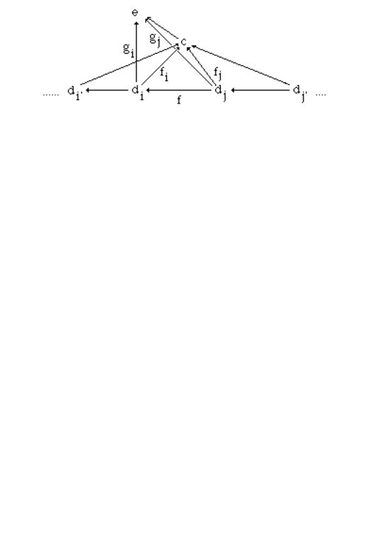
{fi C[c,di] | i I } such that |
i,j I e E fe C[di,dj] fe ° fi = fj .
A cone may be visualized by
Cocones are defined dually.
Example In a partial order P, cones correspond to lower bounds, cocones to upper bounds.
Note now that, given a diagram D, the cones to |
D form a category, call it |
ConesC,D . |
Just take |
as morphisms from (c,{fi C[c,di] | i I}) to |
(c',{hi C[c',di] | i I}) any |
g C[c,c'] |
such that |
i I hi ° g = fi. That is, |
|
|
|
Clearly, ConesC,D is a category. Dually one defines the category CoconesC,D .
6.1.3 Definition. Let C be a category and D a diagram. Then a limit for D is a terminal object in ConesC,D . Colimits are defined dually.
(c,{fi C[di,c] | i I}) is the initial object in CoconesC,D, it may be visualized by the following commutative diagram:
121
6. Cones and Limits
Limits are also called universal cones, as any other cone uniquely factorizes via them. Dually, colimits are called universal cocones.
Examples
1. Let P be a partial order. Then limits correspond to greater lower bounds, while colimits correspond to least upper bounds.
2. Let D = ({di}iω, {fi Set[di, di+1]}iω ) be a diagram in Set such that di di+1, and fi = incl (the set-theoretic inclusion). Then the colimit of d0 →.......di → di+1 →..... is {di}
(exercise: what is the limit of the same diagram?) .
Exercise Prove that the colimits in C are the limits in Cop of the dual diagram.
Consider now a diagram as a functor from an index category I to C. Note first that any object c of the category C is the image of a constant functor Kc: I→C, and so Kc can be regarded as a
degenerate diagram of type I in C. Once diagrams are defined as functors, it makes sense to
consider natural transformations between diagrams. If D and D' are two diagrams of type I, a natural transformation from D to D' is a family of arrows fi indexed on objects in I such that for
each arrow e in I (each edge of the graph of type I)
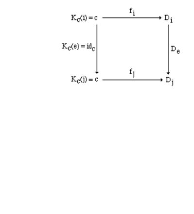
A cone for a diagram D of type I from an object c is then a natural transformation from the constant diagram Kc to D
122
6. Cones and Limits
Dually, a cocone for a diagram D of type I to an object c is a natural transformation from D to the constant diagram Kc .
6.2 Some Constructions Revisited
Let D be an empty diagram, that is a diagram with no objects and no arrows. By definition, a cone in C to D is then just an object c of C, with no other structure (and every object of C can be seen
as a cone). A limit for the empty diagram is then an object t such that for any other object c there is exactly one arrow from c to t, i.e., it is a terminal object. Dually, the initial object is the colimit of the empty diagram.
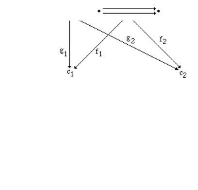
A graph is called discrete if it has no arrows. For example the set {1,2} can be regarded as a discrete graph. A diagram of type {1,2} in a category C is an ordered pair of objects, (c1,c2). A
limit for such a diagram is an object d, together with two arrows f1: d→c1 and f2: d→c2, |
such |
that for any other cone (d',{gi C[d',ci] | i {1,2} }) there exists exactly one arrow h: d'→d, |
with |
fi ° h = gi for i {1,2}. |
|
But this is just the definition of product d of c1 and c2 with f1: d→c1 and f2: d→c2 as
projections.
Dually, the coproduct ci#cj, if it exists, is just the the colimit of the diagram {ci,cj}.
The product of any indexed collection of objects in a category is defined analogously as the limit of the diagram D: I→C where I is the index set considered as a discrete graph. This product is usually denoted by Πi IDi, although explicit mention of the index set is often omitted.
Consider the graph I with two vertices and two edges
A diagram of type |
I in a category C is a pair of objects, a |
and b, and a pair of parallel arrows |
||
f,g C[a,b]. A cone for this diagram consists of an object |
d, |
and two arrows h C[d,a] and |
||
k C[d,b] such that g ° h = k |
and f ° h = k. A limit is a cone |
(d,{h,k}) that is universal, that is, |
||
for any other cone |
(d',{h',k'}) |
there exists exactly one arrow |
l: d'→d such that h ° l = h', and k ° |
|
l = k'. |
|
|
|
|
123