02.State-space representations (the time-domain)

From these observations follow the form of T AT −1 in the theorem statement. Now let us show that the pair

is controllable. First, by direct calculation, we have

Now, by our choice of basis vectors we also have

image(C(T AT −1, T b)) = span {v1, . . . , vj, vj+1, . . . , vj+k} .

That the pair

is observable follows in the same manner as the previous step, noting that

If we write the state vector as x = (x1, x2, x3, x4) in the decomposition given by the theorem then we may roughly say that

1.x1 represents the states that are controllable but not observable,

2.x2 represents the states that are controllable and observable,

3.x3 represents the states that are neither controllable nor observable,

4.x4 represents the states that are observable but not controllable.

2.6 Summary

This is, as we mentioned in the introduction to the chapter, a di cult bit of material. Here’s what you should take away with you, and make sure you are clear on before proceeding.

1.You should know exactly what we mean when we say “SISO linear system.” This terminology will be used constantly in the remainder of the book.

2.You should be able to take a physical system and put it into the form of an SISO linear system if requested to do so. To do this, linearisation may be required.

3.Given a SISO linear system with a specified input u(t), you should know how to determine, both on paper and with the computer, the output y(t) given an initial value x(0) for the state.

4.You should be able to determine whether a SISO linear system is observable or controllable, and know how the lack of observability or controllability a ects a system.

5.You should know roughly the import of ker(O(A, c)) and of the columnspace of C(A, b).

6.You should know that there is a thing called “zero dynamics,” and you should convince yourself that you can work through Algorithm 2.28 to determine this, at least if you had some time to work it out. We will revisit zero dynamics in Section 3.3, and there you will be given an easy way to determine whether the zero dynamics are stable or unstable.

7.You should be able to determine, by hand and with the computer, the impulse response of a SISO linear system. You should also understand that the impulse response is somehow basic in describing the behaviour of the system—this will be amply borne out as we progress through the book.

8.You should know that a controllable pair (A, b) has associated to it a canonical form, and you should be able to write down this canonical form given the characteristic polynomial for A.

Exercises

The next three exercises are concerned with interconnections of SISO linear systems. We shall be discussing system interconnections briefly at the beginning of Chapter 3, and thoroughly in Chapter 6. Indeed system interconnections are essential to the notion of feedback.

E2.1 Consider two SISO linear systems governed by the di erential equations

(

System 1 equations

x˙ 1(t) = A1x1(t) + b1u1(t) y1(t) = ct1x1(t)

(

System 2 equations

x˙ 2(t) = A2x2(t) + b2u2(t) y2(t) = ct2x2(t),

where x1 Rn1 and x2 Rn2 . The input and output signals of System 1, denoted u1(t) and y1(t), respectively, are both scalar. The input and output signals of System 2, denoted u2(t) and y2(t), respectively, are also both scalar. The matrices A1 and A2 and the vectors b1, b2, and c1, and c2 are of appropriate dimension.

Since each system is single-input, single-output we may “connect” them as shown in Figure E2.1. The output of System 1 is fed into the input of System 2 and so the

Figure E2.1 SISO linear systems connected in series

interconnected system becomes a single-input, single-output system with input u1(t) and output y2(t).

(a) Write the state-space equations for the combined system in the form

where you must determine the expressions for A, b, c, and D. Note that the combined state vector is in Rn1+n2 .

(b)What is the characteristic polynomial of the interconnected system A matrix? Does the interconnected system share any eigenvalues with either of the two component systems?

E2.2 Consider again two SISO linear systems governed by the di erential equations

(

System 1 equations

x˙ 1(t) = A1x1(t) + b1u1(t) y1(t) = ct1x1(t)

(

System 2 equations

x˙ 2(t) = A2x2(t) + b2u2(t) y2(t) = ct2x2(t),

where x1 Rn1 and x2 Rn2 . The input and output signals of System 1, denoted u1(t) and y1(t), respectively, are both scalar. The input and output signals of System 2, denoted u2(t) and y2(t), respectively, are also both scalar. The matrices A1 and A2 and the vectors b1, b2, and c1, and c2 are of appropriate dimension.

Since each system is single-input, single-output we may “connect” them as shown in Figure E2.2. The input to both systems is the same, and their outputs are added

System 2

y2(t)

Figure E2.2 SISO linear systems connected in parallel

to get the new output.

(a) Write the state-space equations for the combined system in the form

where you must determine the expressions for A, b, c, and D. Note that the combined state vector is in Rn1+n2 .

(b)What is the characteristic polynomial of the interconnected system A matrix? Does the interconnected system share any eigenvalues with either of the two component systems?

E2.3 Consider yet again two SISO linear systems governed by the di erential equations

(

System 1 equations

x˙ 1(t) = A1x1(t) + b1u1(t) y1(t) = ct1x1(t)

(

System 2 equations

x˙ 2(t) = A2x2(t) + b2u2(t) y2(t) = ct2x2(t),

where x1 Rn1 and x2 Rn2 . The input and output signals of System 1, denoted u1(t) and y1(t), respectively, are both scalar. The input and output signals of System 2, denoted u2(t) and y2(t), respectively, are also both scalar. The matrices A1 and A2 and the vectors b1, b2, and c1, and c2 are of appropriate dimension.

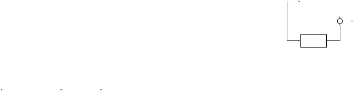
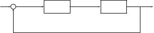
Since each system is single-input, single-output we may “connect” them as shown in Figure E2.3. Thus the input to System 1 is the actual system input u, minus the output from System 2. The input to System 2 is the output from System 1, and the actual system output is the output of System 2.

for p0, p1, . . . , pn−1 R. Show that (A, b) is controllable by verifying that the controllability matrix has full rank.

E2.12 Define (A, c) Rn×n × Rn by

for p0, p1, . . . , pn−1 R. Show that (A, c) is observable by verifying that the observability matrix has full rank.

The next two exercises give conditions for controllability and observability called the Popov- Belevitch-Hautus conditions [see Hautus 1969].

E2.13 Show that (A, b) Rn×n × Rn is controllable if and only if the matrix

(a)Give conditions under which the system is observable.

(b)Give conditions under which the system is controllable.

E2.18 Consider the circuit of Exercise E1.9. Take as output the current emanating from the voltage source (by the Kirchho current law, this is also the sum of the currents through the two resistors).

(a)Give conditions under which the system is observable.

(b)Give conditions under which the system is controllable.

E2.19 For the coupled masses of Exercise E1.4 (assume no damping), suppose you apply a force to the leftmost mass of magnitude F1 = u(t). You also apply a force to the rightmost mass that is proportional to F1; thus you take F2 = αu(t) for some α R. The system is still single-input since the two forces are essentially determined by u(t). As an output for the system take the displacement of the rightmost mass.

(a)Determine for which values of α the system is observable. For those cases when the system is not observable, can you give a physical interpretation of why it is not by looking at ker(O(A, c))?

(b)Determine for which values of α the system is controllable. For those cases when the system is not controllable, can you give a physical interpretation of why it is not by looking at image(C(A, b))?

E2.20 For the pendulum/cart system of Exercises E1.5 and E2.4, determine whether the linearisations in the following cases are observable and/or controllable:

(a)the equilibrium point (0, 0) with cart position as output;

(b)the equilibrium point (0, 0) with cart velocity as output;

(c)the equilibrium point (0, 0) with pendulum angle as output;

(d)the equilibrium point (0, 0) with pendulum angular velocity as output;

(e)the equilibrium point (0, π) with cart position as output;

(f)the equilibrium point (0, π) with cart velocity as output;

(g)the equilibrium point (0, π) with pendulum angle as output;

(h)the equilibrium point (0, π) with pendulum angular velocity as output.

Make sense of your answers by examining ker(C(A, b)) and image(O(A, c)).

E2.21 Consider the the double pendulum of Exercises E1.6 and E2.5. For each of the following cases, determine whether the linearisation is controllable and/or observable:

(a)the equilibrium point (0, 0, 0, 0) with the pendubot input;

(b)the equilibrium point (0, π, 0, 0) with the pendubot input;

(c)the equilibrium point (π, 0, 0, 0) with the pendubot input;

(d)the equilibrium point (π, π, 0, 0) with the pendubot input;

(e)the equilibrium point (0, 0, 0, 0) with the acrobot input;

(f)the equilibrium point (0, π, 0, 0) with the acrobot input;

(g)the equilibrium point (π, 0, 0, 0) with the acrobot input;

(h)the equilibrium point (π, π, 0, 0) with the acrobot input.

In each case, the output is the angle of the second link.

E2.22 Consider the coupled tank system of Exercises E1.11 and E2.6. Determine whether the system is controllable and/or observable for the following outputs:

(a)the output is the level in tank 1;

(b)the output is the level in tank 2;

(c)the output is the di erence in the levels.

E2.23 Determine the zero dynamics for the pendulum/cart system of Exercises E1.5 and E2.4 for each of the following linearisations:

(a)the equilibrium point (0, 0) with cart position as output;

(b)the equilibrium point (0, 0) with cart velocity as output;

(c)the equilibrium point (0, 0) with pendulum angle as output;

(d)the equilibrium point (0, 0) with pendulum angular velocity as output;

(e)the equilibrium point (0, π) with cart position as output;

(f)the equilibrium point (0, π) with cart velocity as output;

(g)the equilibrium point (0, π) with pendulum angle as output;

(h)the equilibrium point (0, π) with pendulum angular velocity as output.

E2.24 For the double pendulum of Exercises E1.6 and E2.5, and for each of the following cases, determine the zero dynamics:

(a)the equilibrium point (0, 0, 0, 0) with the pendubot input;

(b)the equilibrium point (0, π, 0, 0) with the pendubot input;

(c)the equilibrium point (π, 0, 0, 0) with the pendubot input;

(d)the equilibrium point (π, π, 0, 0) with the pendubot input;

(e)the equilibrium point (0, 0, 0, 0) with the acrobot input;

(f)the equilibrium point (0, π, 0, 0) with the acrobot input;

(g)the equilibrium point (π, 0, 0, 0) with the acrobot input;

(h)the equilibrium point (π, π, 0, 0) with the acrobot input.

In each case, use the angle of the second link as output.

E2.25 Determine the linearised zero dynamics of for the coupled tank system of Exercises E1.11 and E2.6 for the following outputs:

(a)the height in tank 1;

(b)the height in tank 2;

(c)the di erence of the heights in the tanks.

E2.26 Define a SISO linear system Σ = (A, b, ct, 01) with

for σ R and ω > 0. Determine the impulse response hΣ(t). Plot the impulse response for various values of σ.

E2.27 Consider the pendulum/cart system of Exercises E1.5 and E2.4, and determine the impulse response of the system for the following linearisations:

(a)the equilibrium point (0, 0) with cart position as output;

(b)the equilibrium point (0, 0) with cart velocity as output;

(c)the equilibrium point (0, 0) with pendulum angle as output;

(d)the equilibrium point (0, 0) with pendulum angular velocity as output;

(e)the equilibrium point (0, π) with cart position as output;

(f)the equilibrium point (0, π) with cart velocity as output;

(g)the equilibrium point (0, π) with pendulum angle as output;

(h)the equilibrium point (0, π) with pendulum angular velocity as output.

E2.28 Select values for the parameters of the double pendulum system of Exercises E1.6 and E2.5. For each of the following cases, determine the impulse response for the linearisation:

(a)the equilibrium point (0, 0, 0, 0) with the pendubot input;

(b)the equilibrium point (0, π, 0, 0) with the pendubot input;

(c)the equilibrium point (π, 0, 0, 0) with the pendubot input;

(d)the equilibrium point (π, π, 0, 0) with the pendubot input;

(e)the equilibrium point (0, 0, 0, 0) with the acrobot input;

(f)the equilibrium point (0, π, 0, 0) with the acrobot input;

(g)the equilibrium point (π, 0, 0, 0) with the acrobot input;

(h)the equilibrium point (π, π, 0, 0) with the acrobot input.

In each case, use the angle of the second link as output.

E2.29 Determine the linearised impulse response for the coupled tank system of Exercises E1.11 and E2.6 for the following outputs:

(a)the height in tank 1;

(b)the height in tank 2;

(c)the di erence of the heights in the tanks.

E2.30 Let

(a)Verify that (A, b) is controllable.

(b)Find the controller canonical form for (A, b).

The next few exercises deal with alternative canonical forms for controllable pairs (A, b) and for observable pairs (A, c).

E2.31 Let (A, b) be a controllable pair. Show that the representations of A and b in the basis {b, Ab, . . . , An−1b} are given by

This is the controllability canonical form or the first Luenberger-Brunovsky canonical form for (A, b).

E2.32 Again let (A, b) be controllable. Recall from Exercise E2.31 that if

E2.34 Let (A, c) be an observable pair. Show that the representations of A and c in the basis formed from the columns of the matrix

This is the observability canonical form or the first Luenberger-Brunovsky canonical form for (A, c).

E2.35 Again let (A, c) be observable. Recall from Exercise E2.34 that if

T 1 = c Atc · · · (At)n−1c ,