

page 27
• What to do when a lot is rejected
time shortage
- Have your employees sort the parts
- have your suppliers employees sort the parts at your facility
image and moral |
- send the parts back to the supplier |
|
important |
||
|
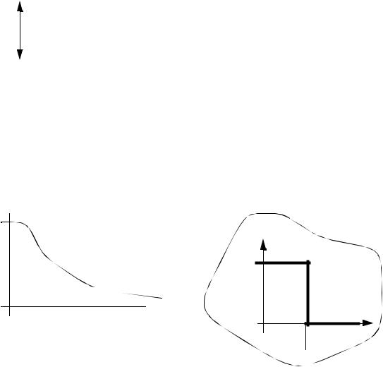
4.5 OPERATING CHARACTERISTIC (OC) CURVES
• Used to estimate the probability of lot rejection, and design sampling plans.
for a single sampled plan |
|
|
|
1 |
|
|
|
N = 3000 |
Pa |
*ideal |
|
n = 89 |
|
|
|
c = 2 |
|
|
|
Pa |
|
|
|
|
|
accept |
reject |
100p0 |
|
|
np0 |
|
|
|
|
Pa - the probability the lot is accepted |
|
AQL |
|
p0 - the fraction of the lot that is nonconforming |
|
|
|
N - the number in the lot |
|
|
|
n - the size of the test sample |
|
|
|
c - the maximum number nonconforming for acceptance |
|
|
|
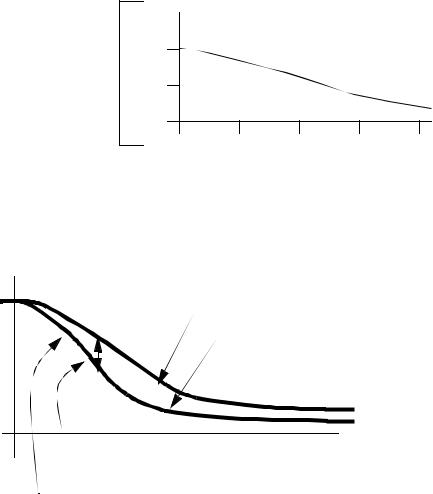
• Drawing the single sampling curve (assuming Poisson distribution)
page 28
|
|
|
|
|
|
|
|
|
|
|
|
|
getting the numbers |
Pa = P0 + P1 + .... + Pn |
|
|
|
|
|
|
|||||
|
or easier use the values in table C |
|
|
|||||||||
|
|
|
|
|
|
|
|
|
|
|
||
******INLCUDE TABLE C OR EQUIVALENT |
|
|
||||||||||
make a table of values |
|
|
|
p0 |
|
100p0 |
|
np0 |
|
|
Pa |
|
|
|
|
|
|
|
|
|
|||||
|
|
|
|
|
|
|||||||
|
|
|
|
|
|
|
|
|
|
|
||
.01 |
|
1 |
|
.9 |
|
|
.938 |
|
||||
|
.02 |
|
2 |
|
1.8 |
|
|
.731 |
|
|||
|
.03 |
|
3 |
|
2.7 |
|
|
.494 |
given |
|||
|
. |
|
. |
|
. |
|
|
. |
||||
|
. |
|
. |
|
. |
|
|
. |
c = 2 |
|||
|
. |
|
. |
|
. |
|
|
. |
n = 89 |
|||
|
|
|
|
|
|
|
|
|
|
|
|
|
graph and |
|
1 |
|
|
|
interpolate |
|
|
|
|
|
Pa |
|
|
|
|
|
|
.5 |
|
|
|
|
|
|
|
|
|
|
|
|
1 |
2 |
3 |
4 |
|
|
|
|
p0 |
|
|
|
|
|
|
• Double sampling curves
accept second sample |
accept first sample |
Pa |
p0 |
calculate added probability
get this curve normally for 1st sample only
page 29
- Assume for the first sample
0 fails |
accept (c1 = 1) |
1 fails |
|
2 fails |
another sample |
3 fails |
|
4 fails |
reject (r1 = 4) |
etc... |
- for the second sample (assume 5 is the upper limit, r2 = 6) for 2 fails in the first sample (Pa2)
∆ Pa = (Pa2)(P3 or less this time)
from first table |
from table C |
|
for 3 fails in the first sample (Pa3)
∆ Pa = (Pa3)(P2 or less this time)
add together for difference
-for multiple sampling, continue from above
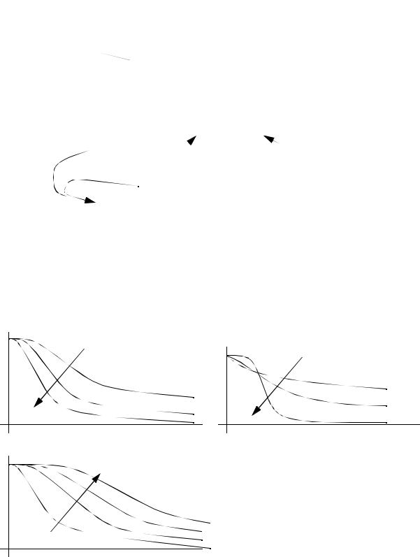
•Factors that vary OC curves
N increases, n α |
N |
c increases |
n increases |
page 30
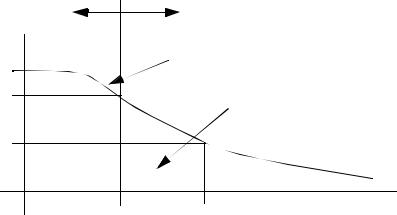
• Producers/Consumers risk |
|
lots above AQL |
lots below AQL |
(should all be accepted) |
(should all be rejected) |
1.0 |
false rejects |
|
|
α |
false accepts |
|
|
β |
|
AQL |
LQL |
α = producers risk of rejection
β = consumers risk of acceptance LQL = Limiting Quality Level AQL = Acceptable Quality Level
• The basic trade-off to be considered when designing sampling plans.
-The producer does not want to have lots with higher rejects than the AQL to be rejected. Typically lots have acceptance levels at 95% when at AQL. This gives a producers risk of α = 100% - 95% = 5%. In real terms this means if products are near the AQL, they have a 5% chance of being rejected even though they are acceptable.
-The consumer/customer does not want to accept clearly unacceptable parts. If the quality is
beyond a second unacceptable limit, the LQL (Lower Quality Level) they will typically be accepted 10% of the time, giving a consumers risk of β = 10%. This limit is also known as the LTPD (Lot Tolerance Percent Defective) or RQL (Rejectable Quality Level).
• AOQ (Average Outgoing Quality)
received quality
cut off at quality level
supplied quality
page 31
with lot-by-lot
acceptance for a manufacturer specified quality level
AOQ |
|
|
|
|
|
average outgoing |
|
AOQL |
|
quality limit |
|
|
|
||
most lots |
some lots |
most lots |
|
rejected |
rejected |
||
accepted |
|||
|
|
• AOQ (Average Outgoing Quality) - a simple relationship between quality shipped and quality accepted.
* Note: this does not account
AOQ = (supplied quality)Pa for discarded units, but is close enough.
• ASN (Average Sample Number) - the number of samples the receiver has to do
page 32
The chance a second sample is taken
ASN = n1 |
Single sample |
ASN = n1 + n2(1-PI) |
Double sample |
ASN |
|
single
double
 multiple
fraction non-conforming (p0)
DESIGNING A SAMPLE PLAN
e.g. when only concerned with the producers risk
1.get producers risk of α (given)
2.get AQL (given)
3.refer to table of values to start (e.g. pg.314)
-given: α =0.5, therefore Pa=.95
-look at c (Pass/Fail sample size)
-for c=1, np = .355
-given AQL = 1.5% = .015
-n = .355/.015 = 23.67 = 24
-for c=5, np=2.613
-n=2.613/.015 = 174.2 = 175
4. Select a sample from acceptable list |
e.g. |
c |
n |
|
|
|
|
|
|
1 |
24 |
|
|
5 |
175 |
•On the other hand, given consumers risk (β ) and Lower Quality Level (LQL), we can follow a similar approach, still using the table on pg. 314
•Given α and AQL, and β and LQL we can also find a best fit plan through trial and error.