

TsOS / DSP_guide_Smith / Ch25
.pdfSNR 0.5
1.0
2.0
Chapter 25Special Imaging Techniques |
433 |

 Pixel value
Column number
Pixel value
Column number
Pixel value
Column number
FIGURE 25-8
Minimum detectable SNR. An object is visible in an image only if its contrast is large enough to overcome the random image noise. In this example, the three squares have SNRs of 2.0, 1.0 and 0.5 (where the SNR is defined as the contrast of the object divided by the standard deviation of the noise).
as the brightness of the ambient lightning, the distance between the two regions being compared, and how the grayscale image is formed (video monitor, photograph, halftone, etc.).
The grayscale transform of Chapter 23 can be used to boost the contrast of a selected range of pixel values, providing a valuable tool in overcoming the limitations of the human eye. The contrast at one brightness level is increased, at the cost of reducing the contrast at another brightness level. However, this only works when the contrast of the object is not lost in random image noise. This is a more serious situation; the signal does not contain enough information to reveal the object, regardless of the performance of the eye.
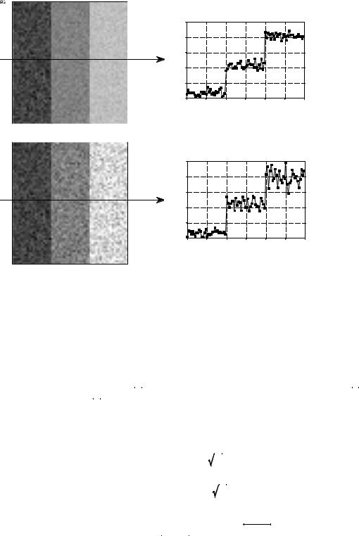
Figure 25-8 shows an image with three squares having contrasts of 5%, 10%, and 20%. The background contains normally distributed random noise with a standard deviation of about 10% contrast. The SNR is defined as the contrast divided by the standard deviation of the noise, resulting in the three squares having SNRs of 0.5, 1.0 and 2.0. In general, trouble begins when the SNR falls below about 1.0.

434 |
The Scientist and Engineer's Guide to Digital Signal Processing |
The exact value for the minimum detectable SNR depends on the size of the object; the larger the object, the easier it is to detect. To understand this, imagine smoothing the image in Fig. 25-8 with a 3×3 square filter kernel. This leaves the contrast the same, but reduces the noise by a factor of three (i.e., the square root of the number of pixels in the kernel). Since the SNR is tripled, lower contrast objects can be seen. To see fainter objects, the filter kernel can be made even larger. For example, a 5×5 kernel improves the SNR by a factor of  25 ' 5 . This strategy can be continued until the filter kernel is equal to the size of the object being detected. This means the ability to detect an object is proportional to the square-root of its area. If an object's diameter is doubled, it can be detected in twice as much noise.
Visual processing in the brain behaves in much the same way, smoothing the viewed image with various size filter kernels in an attempt to recognize low contrast objects. The three profiles in Fig. 25-8 illustrate just how good humans are at detecting objects in noisy environments. Even though the objects can hardly be identified in the profiles, they are obvious in the image. To really appreciate the capabilities of the human visual system, try writing algorithms that operate in this low SNR environment. You'll be humbled by what your brain can do, but your code can't!
Random image noise comes in two common forms. The first type, shown in Fig. 25-9a, has a constant amplitude. In other words, dark and light regions in the image are equally noisy. In comparison, (b) illustrates noise that increases with the signal level, resulting in the bright areas being more noisy than the dark ones. Both sources of noise are present in most images, but one or the other is usually dominant. For example, it is common for the noise to decrease as the signal level is decreased, until a plateau of constant amplitude noise is reached.
A common source of constant amplitude noise is the video preamplifier. All analog electronic circuits produce noise. However, it does the most harm where the signal being amplified is at its smallest, right at the CCD or other imaging sensor. Preamplifier noise originates from the random motion of electrons in the transistors. This makes the noise level depend on how the electronics are designed, but not on the level of the signal being amplified. For example, a typical CCD camera will have an SNR of about 300 to 1000 (40 to 60 dB), defined as the full scale signal level divided by the standard deviation of the constant amplitude noise.
Noise that increases with the signal level results when the image has been represented by a small number of individual particles. For example, this might be the x-rays passing through a patient, the light photons entering a camera, or the electrons in the well of a CCD. The mathematics governing these variations are called counting statistics or Poisson statistics. Suppose that the face of a CCD is uniformly illuminated such that an average of 10,000 electrons are generated in each well. By sheer chance, some wells will have more electrons, while some will have less. To be more exact, the number of electrons will be normally distributed with a mean of 10,000, with some standard deviation that describes how much variation there is from
Chapter 25Special Imaging Techniques |
435 |
a. Constant amplitude noise
Pixel value |
Column number
b. Noise dependent on signal level
Pixel value |
Column number
FIGURE 25-9
Image noise. Random noise in images takes two general forms. In (a), the amplitude of the noise remains constant as the signal level changes. This is typical of electronic noise. In (b), the amplitude of the noise increases as the square-root of the signal level. This type of noise originates from the detection of a small number of particles, such as light photons, electrons, or x-rays.
well-to-well. A key feature of Poisson statistics is that the standard deviation is equal to the square-root of the number of individual particles. That is, if there are N particles in each pixel, the mean is equal to N and the standard deviation is equal to  N . This makes the signal-to-noise ratio equal to N/
 N , or simply,
  N . In equation form:
EQUATION 25-1 |
µ ' N |
|||
Poisson statistics. In a Poisson distributed |
|
|
|
|
signal, the mean, µ, is the average number |
F ' |
|
|
|
of individual particles, N. The standard |
N |
|
||
deviation, F, is equal to the square-root of |
|
|
|
|
the average number of individual particles. |
|
|
|
|
The signal-to-noise ratio (SNR) is the mean |
|
|
|
|
SNR ' |
|
N |
||
divided by the standard deviation. |
|
|||
|
|
|
|
|
In the CCD example, the standard deviation is  10,000 ' 100 . Likewise the signal-to-noise ratio is also
  10,000 ' 100 . If the average number of electrons per well is increased to one million, both the standard deviation and the SNR increase to 1,000. That is, the noise becomes larger as the signal becomes
436 |
The Scientist and Engineer's Guide to Digital Signal Processing |
larger, as shown in Fig. 25-9b. However, the signal is becoming larger faster than the noise, resulting in an overall improvement in the SNR. Don't be confused into thinking that a lower signal will provide less noise and therefore better information. Remember, your goal is not to reduce the noise, but to extract a signal from the noise. This makes the SNR the key parameter.
Many imaging systems operate by converting one particle type to another. For example, consider what happens in a medical x-ray imaging system. Within an x-ray tube, electrons strike a metal target, producing x-rays. After passing through the patient, the x-rays strike a vacuum tube detector known as an image intensifier. Here the x-rays are subsequently converted into light photons, then electrons, and then back to light photons. These light photons enter the camera where they are converted into electrons in the well of a CCD. In each of these intermediate forms, the image is represented by a finite number of particles, resulting in added noise as dictated by Eq. 25-1. The final SNR reflects the combined noise of all stages; however, one stage is usually dominant. This is the stage with the worst SNR because it has the fewest particles. This limiting stage is called the quantum sink.
In night vision systems, the quantum sink is the number of light photons that can be captured by the camera. The darker the night, the noisier the final image. Medical x-ray imaging is a similar example; the quantum sink is the number of x-rays striking the detector. Higher radiation levels provide less noisy images at the expense of more radiation to the patient.
When is the noise from Poisson statistics the primary noise in an image? It is dominant whenever the noise resulting from the quantum sink is greater than the other sources of noise in the system, such as from the electronics. For example, consider a typical CCD camera with an SNR of 300. That is, the noise from the CCD preamplifier is 1/300th of the full scale signal. An equivalent noise would be produced if the quantum sink of the system contains 90,000 particles per pixel. If the quantum sink has a smaller number of particles, Poisson noise will dominate the system. If the quantum sink has a larger number of particles, the preamplifier noise will be predominant. Accordingly, most CCD's are designed with a full well capacity of 100,000 to 1,000,000 electrons, minimizing the Poisson noise.
Morphological Image Processing
The identification of objects within an image can be a very difficult task. One way to simplify the problem is to change the grayscale image into a binary image, in which each pixel is restricted to a value of either 0 or 1. The techniques used on these binary images go by such names as: blob analysis, connectivity analysis, and morphological image processing
(from the Greek word morphe, meaning shape or form). The foundation of morphological processing is in the mathematically rigorous field of set theory; however, this level of sophistication is seldom needed. Most morphological algorithms are simple logic operations and very ad hoc. In
Chapter 25Special Imaging Techniques |
437 |
|
a. Original |
b. Erosion |
c. Dilation |
d. Opening |
e. Closing |
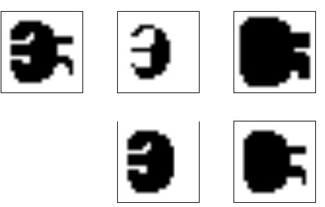
FIGURE 25-10
Morphological operations. Four basic morphological operations are used in the processing of binary images: erosion, dilation, opening, and closing. Figure (a) shows an example binary image. Figures
(b) to (e) show the result of applying these operations to the image in (a).
other words, each application requires a custom solution developed by trial- and-error. This is usually more of an art than a science. A bag of tricks is used rather than standard algorithms and formal mathematical properties. Here are some examples.
Figure 25-10a shows an example binary image. This might represent an enemy tank in an infrared image, an asteroid in a space photograph, or a suspected tumor in a medical x-ray. Each pixel in the background is displayed as white, while each pixel in the object is displayed as black. Frequently, binary images are formed by thresholding a grayscale image; pixels with a value greater than a threshold are set to 1, while pixels with a value below the threshold are set to 0. It is common for the grayscale image to be processed with linear techniques before the thresholding. For instance, illumination flattening (described in Chapter 24) can often improve the quality of the initial binary image.
Figures (b) and (c) show how the image is changed by the two most common morphological operations, erosion and dilation. In erosion, every object pixel that is touching a background pixel is changed into a background pixel. In dilation, every background pixel that is touching an object pixel is changed into an object pixel. Erosion makes the objects smaller, and can break a single object into multiple objects. Dilation makes the objects larger, and can merge multiple objects into one.
As shown in (d), opening is defined as an erosion followed by a dilation. Figure (e) shows the opposite operation of closing, defined as a dilation followed by an erosion. As illustrated by these examples, opening removes small islands and thin filaments of object pixels. Likewise, closing removes
438 |
The Scientist and Engineer's Guide to Digital Signal Processing |
islands and thin filaments of background pixels. These techniques are useful for handling noisy images where some pixels have the wrong binary value. For instance, it might be known that an object cannot contain a "hole", or that the object's border must be smooth.
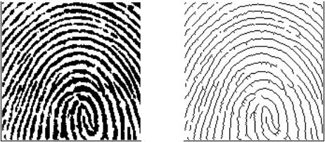
Figure 25-11 shows an example of morphological processing. Figure (a) is the binary image of a fingerprint. Algorithms have been developed to analyze these patterns, allowing individual fingerprints to be matched with those in a database. A common step in these algorithms is shown in (b), an operation called skeletonization. This simplifies the image by removing redundant pixels; that is, changing appropriate pixels from black to white. This results in each ridge being turned into a line only a single pixel wide.
Tables 25-1 and 25-2 show the skeletonization program. Even though the fingerprint image is binary, it is held in an array where each pixel can run from 0 to 255. A black pixel is denoted by 0, while a white pixel is denoted by 255. As shown in Table 25-1, the algorithm is composed of 6 iterations that gradually erode the ridges into a thin line. The number of iterations is chosen by trial and error. An alternative would be to stop when an iteration makes no changes.
During an iteration, each pixel in the image is evaluated for being removable; the pixel meets a set of criteria for being changed from black to white. Lines 200-240 loop through each pixel in the image, while the subroutine in Table 25-2 makes the evaluation. If the pixel under consideration is not removable, the subroutine does nothing. If the pixel is removable, the subroutine changes its value from 0 to 1. This indicates that the pixel is still black, but will be changed to white at the end of the iteration. After all the pixels have been evaluated, lines 260-300 change the value of the marked pixels from 1 to 255. This two-stage process results in the thick ridges being eroded equally from all directions, rather than a pattern based on how the rows and columns are scanned.
a. Original fingerprint |
b. Skeletonized fingerprint |
FIGURE 25-11
Binary skeletonization. The binary image of a fingerprint, (a), contains ridges that are many pixels wide. The skeletonized version, (b), contains ridges only a single pixel wide.
|
Chapter 25Special Imaging Techniques |
439 |
|
100 |
'SKELETONIZATION PROGRAM |
|
|
110 |
'Object pixels have a value of 0 (displayed as black) |
|
|
120 |
'Background pixels have a value of 255 (displayed as white) |
|
|
130 |
' |
|
|
140 |
DIM X%[149,149] |
'X%[ , ] holds the image being processed |
|
150 |
' |
|
|
160 |
GOSUB XXXX |
'Mythical subroutine to load X%[ , ] |
|
170 |
' |
|
|
180 |
FOR ITER% = 0 TO 5 |
'Run through six iteration loops |
|
190 |
' |
|
|
200 |
FOR R% = 1 TO 148 |
'Loop through each pixel in the image. |
|
210 |
FOR C% = 1 TO 148 |
'Subroutine 5000 (Table 25-2) indicates which |
|
220 |
GOSUB 5000 |
'pixels can be changed from black to white, |
|
230 |
NEXT C% |
'by marking the pixels with a value of 1. |
|
240 |
NEXT R% |
|
|
250 |
' |
|
|
260 |
FOR R% = 0 TO 149 |
'Loop through each pixel in the image changing |
|
270 |
FOR C% = 0 TO 149 |
'the marked pixels from black to white. |
|
280 |
IF X%(R%,C%) = 1 THEN X%(R%,C%) = 255 |
|
|
290 |
NEXT C% |
|
|
300 |
NEXT R% |
|
|
310 |
' |
|
|
320 NEXT ITER% |
|
|
|
330 |
' |
|
|
340 END |
TABLE 25-1 |
|
|
|
|
|
|
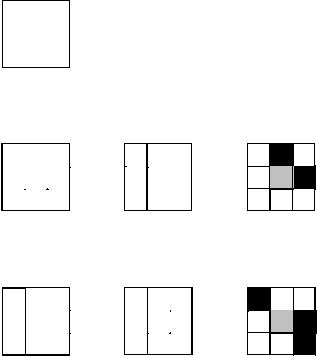
The decision to remove a pixel is based on four rules, as contained in the subroutine shown in Table 25-2. All of these rules must be satisfied for a pixel to be changed from black to white. The first three rules are rather simple, while the fourth is quite complicated. As shown in Fig. 25-12a, a pixel at location [R,C] has eight neighbors. The four neighbors in the horizontal and vertical directions (labeled 2,4,6,8) are frequently called the close neighbors. The diagonal pixels (labeled 1,3,5,7) are correspondingly called the distant neighbors. The four rules are as follows:
Rule one: The pixel under consideration must presently be black. If the pixel is already white, no action needs to be taken.
Rule two: At least one of the pixel's close neighbors must be white. This insures that the erosion of the thick ridges takes place from the outside. In other words, if a pixel is black, and it is completely surrounded by black pixels, it is to be left alone on this iteration. Why use only the close neighbors, rather than all of the neighbors? The answer is simple: running the algorithm both ways shows that it works better. Remember, this is very common in morphological image processing; trial and error is used to find if one technique performs better than another.
Rule three: The pixel must have more than one black neighbor. If it has only one, it must be the end of a line, and therefore shouldn't be removed.
Rule four: A pixel cannot be removed if it results in its neighbors being disconnected. This is so each ridge is changed into a continuous line, not a group of interrupted segments. As shown by the examples in Fig. 25-12,
440 |
The Scientist and Engineer's Guide to Digital Signal Processing |
a. Pixel numbering
Column
|
|
C!1 |
C |
C+1 |
R!1 |
1 |
2 |
3 |
|
Row |
|
|
|
|
R |
8 |
|
4 |
|
|
|
|||
|
|
|
|
|
R+1 |
7 |
6 |
5 |
|
|
|
|
|
|
FIGURE 25-12
Neighboring pixels. A pixel at row and column [R,C] has eight neighbors, referred to by the numbers in (a). Figures (b) and (c) show examples where the neighboring pixels are connected and unconnected, respectively. This definition is used by rule number four of the skeletonization algorithm.
b. Connected neighbors
|
|
|
Column |
|
|
|
|
Column |
||||
|
|
|
C!1 C C+1 |
|
|
|
|
C!1 * C |
C+1 |
|||
R!1 |
|
|
|
|
R!1 |
|
|
|
||||
Row |
|
|
|
|
|
* |
Row |
R |
|
|
|
|
R |
|
|
|
|
|
|||||||
|
|
|
|
|
|
|||||||
|
|
|
|
|
|
|
|
|||||
|
|
|
|
|
|
|
|
|
|
|
||
R+1 |
|
|
|
R+1 |
|
|
||||||
|
|
|
|
|
|
|
|
|
|
|
|
|
|
C!1 |
Column |
|
|
C |
C+1 |
|
R!1 |
|
|
|
Row |
R |
|
|
|
|
|
|
R+1 |
|
* |
|
|
|
||
c. Unconnected neighbors
|
|
|
Column |
|
|
|
C!1 |
Column |
||||||
|
|
|
C!1 |
* C |
C+1 |
|
|
|
|
C C+1 |
||||
R!1 |
|
|
|
|
R!1 |
|
|
|
|
|||||
Row |
|
|
|
|
|
|
Row |
|
|
|
|
|
|
|
R |
|
|
|
|
R |
|
|
|
|
|||||
|
|
|
|
|
|
|
|
|
||||||
|
|
|
|
|
* |
|
* |
|
|
|
|
|
* |
|
R+1 |
|
|
|
|
|
|
|
|
||||||
|
|
R+1 |
|
|
|
|
|
|||||||
|
|
|
|
|
|
|
|
|
|
|
|
|
|
|
Column
C!1 * C C+1
R!1
Row R
* 

R+1
*
connected means that all of the black neighbors touch each other. Likewise, unconnected means that the black neighbors form two or more groups.
The algorithm for determining if the neighbors are connected or unconnected is based on counting the black-to-white transitions between adjacent neighboring pixels, in a clockwise direction. For example, if pixel 1 is black and pixel 2 is white, it is considered a black-to-white transition. Likewise, if pixel 2 is black and both pixel 3 and 4 are white, this is also a black-to-white transition. In total, there are eight locations where a black-to-white transition may occur. To illustrate this definition further, the examples in (b) and (c) have an asterisk placed by each black-to-white transition. The key to this algorithm is that there will be exactly one black-to-white transition if the neighbors are connected. More than one such transition indicates that the neighbors are unconnected.
As additional examples of binary image processing, consider the types of algorithms that might be useful after the fingerprint is skeletonized. A disadvantage of this particular skeletonization algorithm is that it leaves a considerable amount of fuzz, short offshoots that stick out from the sides of longer segments. There are several different approaches for eliminating these artifacts. For example, a program might loop through the image removing the pixel at the end of every line. These pixels are identified
Chapter 25Special Imaging Techniques |
441 |
5000 ' Subroutine to determine if the pixel at X%[R%,C%] can be removed.
5010 ' If all four of the rules are satisfied, then X%(R%,C%], is set to a value of 1, 5020 ' indicating it should be removed at the end of the iteration.
5030 '
5040 'RULE #1: Do nothing if the pixel already white 5050 IF X%(R%,C%) = 255 THEN RETURN
5060 '
5070 '
5080 'RULE #2: Do nothing if all of the close neighbors are black 5090 IF X%[R% -1,C% ] <> 255 AND X%[R% ,C%+1] <> 255 AND
X%[R%+1,C% ] <> 255 AND X%[R% ,C% -1] <> 255 THEN RETURN
5100 '
5110 '
5120 'RULE #3: Do nothing if only a single neighbor pixel is black 5130 COUNT% = 0
5140 IF X%[R% -1,C% -1] |
= 0 THEN COUNT% = COUNT% + 1 |
|
5150 IF X%[R% -1,C% ] |
= 0 THEN COUNT% = COUNT% + 1 |
|
5160 IF X%[R% -1,C%+1] = 0 THEN COUNT% = COUNT% + 1 |
||
5170 IF X%[R% ,C%+1] = 0 THEN COUNT% = COUNT% + 1 |
||
5180 IF X%[R%+1,C%+1] = 0 THEN COUNT% = COUNT% + 1 |
||
5190 IF X%[R%+1,C% ] |
= 0 THEN COUNT% = COUNT% + 1 |
|
5200 IF X%[R%+1,C% -1] |
= 0 THEN COUNT% = COUNT% + 1 |
|
5210 IF X%[R% ,C% -1] |
= 0 THEN COUNT% = COUNT% + 1 |
|
5220 IF COUNT% = 1 THEN RETURN |
|
|
5230 ' |
|
|
5240 ' |
|
|
5250 'RULE 4: Do nothing if the neighbors are unconnected. |
|
|
5260 'Determine this by counting the black-to-white transitions |
|
|
5270 'while moving clockwise through the 8 neighboring pixels. |
||
5280 COUNT% = 0 |
|
|
5290 IF X%[R% -1,C% -1] = 0 AND X%[R% -1,C% ] |
> 0 THEN COUNT% = COUNT% + 1 |
|
5300 IF X%[R% -1,C% ] = 0 AND X%[R% -1,C%+1] |
> 0 AND X%[R% ,C%+1] > 0 |
|
THEN COUNT% = COUNT% + 1 |
|
|
5310 IF X%[R% -1,C%+1] |
= 0 AND X%[R% ,C%+1] |
> 0 THEN COUNT% = COUNT% + 1 |
5320 IF X%[R% ,C%+1] |
= 0 AND X%[R%+1,C%+1] |
> 0 AND X%[R%+1,C% ] > 0 |
THEN COUNT% = COUNT% + 1 |
|
|
5330 IF X%[R%+1,C%+1] |
= 0 AND X%[R%+1,C% ] |
> 0 THEN COUNT% = COUNT% + 1 |
5340 IF X%[R%+1,C% ] |
= 0 AND X%[R%+1,C% -1] |
> 0 AND X%[R% ,C%-1] > 0 |
THEN COUNT% = COUNT% + 1 |
|
|
5350 IF X%[R%+1,C% -1] |
= 0 AND X%[R% ,C% -1] |
> 0 THEN COUNT% = COUNT% + 1 |
5360 IF X%[R% ,C% -1] |
= 0 AND X%[R% -1,C% -1] |
> 0 AND X%[R%-1,C% ] > 0 |
THEN COUNT% = COUNT% + 1 5370 IF COUNT% > 1 THEN RETURN 5380 ' 5390 '
5400 'If all rules are satisfied, mark the pixel to be set to white at the end of the iteration 5410 X%(R%,C%) = 1
5420 '
5430 RETURN
TABLE 25-2
by having only one black neighbor. Do this several times and the fuzz is removed at the expense of making each of the correct lines shorter. A better method would loop through the image identifying branch pixels (pixels that have more than two neighbors). Starting with each branch pixel, count the number of pixels in each offshoot. If the number of pixels in an offshoot is less than some value (say, 5), declare it to be fuzz, and change the pixels in the branch from black to white.
442 |
The Scientist and Engineer's Guide to Digital Signal Processing |
Another algorithm might change the data from a bitmap to a vector mapped format. This involves creating a list of the ridges contained in the image and the pixels contained in each ridge. In the vector mapped form, each ridge in the fingerprint has an individual identity, as opposed to an image composed of many unrelated pixels. This can be accomplished by looping through the image looking for the endpoints of each line, the pixels that have only one black neighbor. Starting from the endpoint, each line is traced from pixel to connecting pixel. After the opposite end of the line is reached, all the traced pixels are declared to be a single object, and treated accordingly in future algorithms.
Computed Tomography
A basic problem in imaging with x-rays (or other penetrating radiation) is that a two-dimensional image is obtained of a three-dimensional object. This means that structures can overlap in the final image, even though they are completely separate in the object. This is particularly troublesome in medical diagnosis where there are many anatomic structures that can interfere with what the physician is trying to see. During the 1930's, this problem was attacked by moving the x-ray source and detector in a coordinated motion during image formation. From the geometry of this motion, a single plane within the patient remains in focus, while structures outside this plane become blurred. This is analogous to a camera being focused on an object at 5 feet, while objects at a distance of 1 and 50 feet are blurry. These related techniques based on motion blurring are now collectively called classical tomography. The word tomography means "a picture of a plane."
In spite of being well developed for more than 50 years, classical tomography is rarely used. This is because it has a significant limitation: the interfering objects are not removed from the image, only blurred. The resulting image quality is usually too poor to be of practical use. The long sought solution was a system that could create an image representing a 2D slice through a 3D object with no interference from other structures in the 3D object.
This problem was solved in the early 1970s with the introduction of a technique called computed tomography (CT). CT revolutionized the medical x-ray field with its unprecedented ability to visualize the anatomic structure of the body. Figure 25-13 shows a typical medical CT image. Computed tomography was originally introduced to the marketplace under the names Computed Axial Tomography and CAT scanner. These terms are now frowned upon in the medical field, although you hear them used frequently by the general public.
Figure 25-14 illustrates a simple geometry for acquiring a CT slice through the center of the head. A narrow pencil beam of x-rays is passed from the x-ray source to the x-ray detector. This means that the measured value at the detector is related to the total amount of material placed anywhere