184 Ship Design for Efficiency and Economy

Relative rotative efficiency

Theoretically, the relative rotative efficiency R accounts for the differences between the open-water test and the inhomogeneous three-dimensional propeller inflow encountered in a propulsion test. In reality, the propeller efficiency behind the ship cannot be measured and all effects not included in the hull efficiency, i.e. wake and thrust deduction fraction, are included in R. In addition, the partial recovery of rotational energy by the rudder contributes to R. This mixture of effects makes it difficult to express R as a function of a few defined parameters.

Holtrop and Mennen (1978) and Holtrop (1984) give

R D 0:9922 0:05908 AE=A0 C 0:07424 .CP 0:0225 lcb/ for single-screw ships

R D 0:9737 C 0:111 .CP 0:0225 lcb/ 0:06325 P=DP for twin-screw ships

lcb is here the longitudinal centre of buoyancy taken from Lwl=2 in [%Lwl] AE=A0 is the blade area ratio of the propeller

P=DP is the pitch-to-diameter ratio of the propeller

Helm (1980) gives for small ships:

LB

R D 0:826 C 0:01 r1=3 C 0:02 T C 0:1 CM

The basis is the same as for Helm's formula for H.

R D 1 0:05 for propeller propulsion systems; Alte and Baur (1986) recommend, as a simple estimate, R D 1:00 for single-screw ships, R D 0:98 for twin-screw ships.

Jensen (1994) gives R D 1:02±1.06 for single-screw ships depending also on details of the experimental and correlation procedure.

6.2 Power prognosis using the admiralty formula

The `admiralty formula' is still used today, but only for a very rough estimate:

12=3 V3

PB D

C

The admiralty constant C is assumed to be constant for similar ships with similar Froude numbers, i.e. ships that have almost the same CB, CP, r=L, Fn, r, etc. Typical values for C in [t2=3 kn3=kW] are:

Ship propulsion 185

These values give an order of magnitude only. The constant C should be determined individually for basis ships used in design. Volker¨ (1974) gives a modified admiralty formula for cargo ships with smaller scatter for C:

10:567 V3:6

PD D

C D

D in this formula may be estimated by one of the above-mentioned empirical formulae. Strictly speaking, the exponent of V should be a function of speed range and ship hull form. The admiralty formula is thus only useful if a ship of the same type, size and speed range is selected to determine C. It is possible to increase the accuracy of the Volker¨ formula by adjusting it to specific ship types.

More accurate methods to estimate the power requirements estimate the resistance as described below:

PB D

RT V

D S

MacPherson (1993) provides some background and guidance to designers for simple computer-based prediction methods, and these are recommended for further studies.

6.3 Ship resistance under trial conditions

Decomposition of resistance

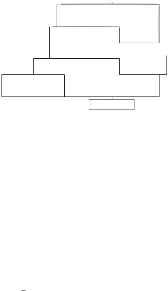
As the resistance of a full-scale ship cannot be measured directly, our knowledge about the resistance of ships comes from model tests. The measured calm-water resistance is usually decomposed into various components, although all these components usually interact and most of them cannot be measured individually. The concept of resistance decomposition helps in designing the hull form as the designer can focus on how to influence individual resistance components. Larsson and Baba (1996) give a comprehensive overview of modern methods of resistance decomposition (Fig. 6.1).

The total calm-water resistance of a new ship hull can be decomposed as

RT D RF C RW C RPV

It is customary to express the resistance by a non-dimensional coefficient, e.g.

RT

CT D =2 V2 S

S is the wetted surface, usually taken at calm-water conditions, although this is problematic for fast ships.

Empirical formulae to estimate S are:

For cargo ships and ferries (Lap, 1954):

S D r1=3 .3:4 r1=3 C 0:5 LWL/

186 Ship Design for Efficiency and Economy

Total Resistance RT

Figure 6.1 Decomposition of ship resistance components

For cargo ships and ferries (Danckwardt, 1969):

For modern warships (Schneekluth, 1988):

S D L .1:8 T C CB B/

Friction resistance

The friction resistance is usually estimated taking the resistance of an `equivalent' flat plate of the same area and length as reference:

RF D CF V2 S

2

CF D 0:075=.log Rn 2/2 according to ITTC 1957. The ITTC formula for CF includes not only the flat plate friction, but also some form and roughness effects. CF is a function of speed, shiplength, temperature and viscosity of the water. However, the speed dependence is almost negligible. For low speeds, friction resistance dominates. The designer will then try to keep the wetted surface S small. This results in rather low L=B and L=T ratios for bulkers and tankers.

Ship propulsion 187

Viscous pressure resistance

A deeply submerged model of a ship will have no wave resistance. But its resistance will be higher than just the frictional resistance. The form of the ship induces a local flow field with velocities that are sometimes higher and sometimes lower than the average velocity. The average of the resulting shear stresses is then higher. Also, energy losses in the boundary layer, vortices and flow separation prevent an increase to stagnation pressure in the aftbody as predicted in an ideal fluid theory. The viscous pressure resistance increases with fullness of waterplane and block coefficient.

An empirical formula for the viscous pressure resistance coefficient is (Schneekluth, 1988):

!

.CP C 58 Cr 0:408/ .0:535 35 Cr/

where Cr D r=L3. The formula was derived from the Taylor experiments based on B=T D 2:25±4:5, CP D 0:48±0:8, Cr D 0:001±0:007.

This viscous pressure resistance is often written as a function of the friction resistance:

RPV D k RF

This so-called form factor approach does not properly include the separation effects. For slender ships, e.g. containerships, the resistance due to separation is negligible (Jensen, 1994). For some icebreakers, inland vessels and other ships with very blunt bows, the form factor approach appears to be inappropriate.

There are various formulae to estimate k:

The viscous pressure resistance depends on the local shape and CFD can be used to improve this resistance component.

Wave resistance

The ship creates a typical wave system which contributes to the total resistance. For fast, slender ships this component dominates. In addition, there are breaking waves at the bow which dominate for slow, full hulls, but may also be considerable for fast ships. The interaction of various wave systems is complicated leading to non-monotonous function of the wave resistance coefficient CW. The wave resistance depends strongly on the local shape. Very general guidelines (see Sections 2.2 to 2.4, 2.9) and CFD (see Section 2.11) are used to improve wave resistance. Slight form changes may result in considerable improvements. This explains the margins of uncertainties for

188 Ship Design for Efficiency and Economy

simple predictions of ship total resistance based on a few parameters as described below.

Prediction methods

Design engineers need simple and reasonably accurate estimates of the power requirements of a ship. Such methods focus on the prediction of the resistance. Some of the older methods listed below are still in use

`Ayre' for cargo ships, Remmers and Kempf (1949)

`Taggart' for tugboats

`Series-60' for cargo ships, Todd et al. (1957)

`BSRA' for cargo ships, Moor et al. (1961)

`Danckwardt' for cargo ships and trawlers, Danckwardt (1969)

`Helm' for small ships, Helm (1964)

`Lap±Keller' for cargo ships and ferries, Lap (1954), Keller (1973)

The following methods have general applicability:

`Taylor±Gertler' (for slender ships), Gertler (1954)

`Guldhammer±Harvald', Guldhammer and Harvald (1974)

`Holtrop±Mennen', Holtrop and Mennen (1978, 1982), Holtrop (1977, 1978, 1984)

`SSPA', Williams (1969)

`Hollenbach', Hollenbach (1997, 1998)

The older methods usually do not consider a bulbous bow. The effect of a bulbous bow may then be approximately introduced by increasing the length in the calculation by 2/3 of the bulb length.

Tables 6.1 to 6.8 show an overview of some of the older methods. The resistance of modern ships is usually higher than predicted by the above methods. The reason is that the following modern form details increase resistance:

Stern bulb.

Hollow waterlines in the vicinity of the upper propeller blades to reduce thrust deduction.

Large propeller aperture to reduce propeller induced vibrations.

Immersed transom stern.

Very broad stern to accommodate a stern ramp in ro-ro ships or to increase stability.

V sections in the forebody of containerships to increase deck area.

Compromises in the location of the shoulders to increase container stowage capacity.

The first two items improve propulsive efficiency. Thus power requirements may be lower despite higher resistance.

The next section describes briefly Hollenbach's method, as this is the most modern, easily programmed and at least as good as the above for modern hull forms.

Ship propulsion 189

Table 6.1 Resistance procedure `Ayre'

Year published: 1927, 1948

Basis for procedure: Evaluation of test results and trials

Description of main value

C D 10:64 V3=PE as f.Fn; L=11=3/

Target value

Effective power PE [HP]

Input values

p

Lpp, Fn D V= g Lpp; 10:64, L=11=3; CB;pp, B=T; lcb, Lwl

Range of variation of input values

Lpp > 30 m; 0:1 Fn 0:3; 0:53 CB;PP 0:85; 2:5%L lcb 2%L

Remarks

1.Influence of bulb not taken into account.

2.Included in the procedure are:

(a)friction resistance using Froude

(b)8% additions for wind and appendages

(c)relating to trial conditions.

3.The procedure is not applicable for Fn > 0:3 and usually yields higher values than other calculation methods.

4.Area of application: Cargo ships.

5.Constant or dependent variable values: D f.Fn/.

References

WENDEL, K. (1954). Angenaherte¨ Bestimmung der notwendigen Maschinenleistung. Handbuch der Werften, p. 34

190 Ship Design for Efficiency and Economy

Table 6.2 Resistance procedure `Taylor-Gertler'

Year published: 1910, 1954, 1964

Basis for procedure: Systematic model tests with a model warship (Royal Navy armoured cruiser Leviathan)

Range of variation of input values

1.Gertler :

0:15 Fn 0:58; 2:25 B=T 3:75; 0:48 CP 0:86; 0:001 r=Lwl3 0:007

2.Rostock :

0:15 Fn 0:33; 2:25 B=T 3:75; 0:48 CP 0:86; 0:002 r=Lwl3 0:007

Remarks

1.Influence of bulb not taken into account.

2.The procedure generally underestimates by 5±10%.

3.Area of application: fast cargo ships, warships.

4.Constant or dependent variable values: CM D 0:925 D constant, Cm D constant, lcb D 0:5Lwl.

References

GERTLER, M. (1954). A reanalysis of the original test data for the Taylor standard series. DTMB report 806, Washington

KRAPPINGER, O. (1963). Schiffswiderstand und Propulsion. Handbuch der Werften, Vol. VII, p. 118

HENSCHKE, W. (1957). Schiffbautechnisches Handbuch Vol. 1, p. 353

¨ . and . (1964). Systematische Widerstandsversuche mit Taylor-Modellen mit

HAHNEL, G LABES, K. H

einem Breiten-Tiefgangsverhaltnis¨ B/T D 4:50. Schiffbauforschung, p. 123

Ship propulsion 191

Table 6.3 Resistance procedure `Lap±Keller'

Year published: 1954, 1973

Basis for procedure: Evaluation of resistance tests (non-systematic) conducted at MARIN (Netherlands)

Description of main value: Resistance coefficient CR D RR=.. =2/ V2 S as f(Group [lcb; p

CP], Number of screws and B=T, V= CP Lpp)

Target value: Residual resistance RR

p

Input values: Lpp; lcb; CP; V= CP Lpp; Number of screws; B=T; AM D CM B T S

Range of variation of input values

p

0:4 V= CP Lpp 1:5; 0:55 CP 0:85; 4% lcb=Lpp 2%

Remarks

1.Influence of bulb not taken into account.

2.The procedure is highly reliable for the region specified.

3.Area of application: cargo and passenger ships

References

LAP, A. J. W. (1954). Diagrams for determining the resistance of single-screw ships. International Shipbuilding Progress, p. 179

HENSCHKE, W. (1957). Schiffbautechnisches Handbuch Vol. 2, p. 129, p. 279

KELLER, W. H. auf'm (1973). Extended diagrams for determining the resistance and required power for single-screw ships. International Shipbuilding Progress, p. 133

192 Ship Design for Efficiency and Economy

Table 6.4 Resistance procedure `Danckwardt'

Year published: 1969

Basis for procedure: Evaluation of model test series and individual tests

ABT (section area at forward perpendicular); S Lpp=r

Range of variation of input values

Cargo and pass. ships: 6 L=B 8; 0:14 Fn 0:32; 2 B=T 3; 0:525 CB 0:825; 50 m Lpp 280 m; 5°C t° 30°C; 0:01 ABT=AM 0:15

Stern trawlers

4 L=B 7; 0:1 Fn 0:36; 2 B=T 3; 0:55 CP 0:7; 25 m Lpp 100 m;0:05Lpp lcb 0

Remarks

1.Influence of bulb taken into account.

2.The procedure is highly reliable for the region specified.

3.Area of application: cargo and passenger ships, stern trawlers.

4.The 1 in the expression RT=1 is a weight `force' of the ship, i.e. displacement mass times gravity acceleration.

References

DANCKWARDT, E. C. M. (1969). Ermittlung des Widerstands von Frachtschiffen und Hecktrawlern beim Entwurf. Schiffbauforschung, p. 124, Errata p. 288

DANCKWARDT, E. C. M. (1981). Algorithmus zur Ermittlung des Widerstands von Hecktrawlern.

Seewirtschaft, p. 551

DANCKWARDT, E. C. M. (1985). Algorithmus zur Ermittlung des Widerstands von Frachtschiffen.

Seewirtschaft, p. 390

DANCKWARDT, E. C. M. (1985). Weiterentwickeltes Verfahren zur Vorausberechnung des Widerstandes von Frachtschiffen. Seewirtschaft, p. 136

Ship propulsion 193

Table 6.5 Resistance procedure `Series-60', Washington

Year published: 1951±1960

Basis for procedure: Systematic model tests with variations of five basic forms. Each basic form represents a block coefficient between 0.6 and 0.8. The basic form for CB D 0:8 was specially designed for this purpose. The other basic forms were based on existing ships.

Range of variation of input values

5:5 L=B 8:5; 0:6 CB;pp 0:8; 2:5 B=T 3:5; 1:2 K 2:4; 45 m Lpp 330 m

Remarks

1.Influence of bulb not taken into account.

2.In addition to resistance, propulsion, partial loading, trim and stern form were also investigated. This is the main advantage of this procedure.

3.Area of application: Cargo ships, tankers

4.Dependent values; constant or variable lcbD f.CB;pp/ and CM D f.CB;pp/

5.The investigated forms differ considerably from modern hull forms.

The ship forms do not represent modern ship hulls. The greatest value of these series from today's view lies in the investigation of partial loading, trim and propulsion.

References

Transactions of the Society of Naval Architects and Marine Engineers 1951, 1953, 1954, 1956, 1957, 1960

Handbuch der Werften Vol. VII, p. 120

HENSCHKE, W. (1957), Schiffbautechnisches Handbuch Vol. 2, pp. 135, 287

SABIT, A. S. (1972). An analysis of the Series 60 results, Part 1, Analysis of form and resistance results. International Shipbuilding Progress, p. 81

SABIT, A. S. (1972). An analysis of the Series 60 results, Part 2, Regression analysis of the propulsion factors. International Shipbuilding Progress, p. 294

194 Ship Design for Efficiency and Economy

Table 6.6 Resistance procedure `SSPA', Gothenborg

Year published: 1948±1959 (summarized 1969)

Basis for procedure: Systematic model tests with ships of selected block coefficients

Description of main value

1.Residual resistance coefficient: CR D RR=.. =2/ V2 S/ as f.CB;pp; L=r1=3; Fn/.

2.Friction resistance coefficient: CF D RF=.. =2/ V2 S/ as Vkn, Lpp.

3.Effective power [HP] as f.V; CB;pp; r; L=r1=3; Lpp/.

Target value: Total resistance Rt [kp]

Input values

p

Lpp; CB;pp; r; Fn D V= g Lpp; L=r1=3

Range of variation of input values

0:525 CB;pp 0:75; 1:5 B=T 6:5; 80 m Lpp 220 m 0:18 Fn 0:32; 5

L=r1=3 7

Remarks

1.Influence of bulb not taken into account.

2.The second reference gives propulsion results.

3.Area of application: cargo ships, passenger ships.

4.Dependent values; constant or variable lcbD f.CB;pp/ and CM D f.CB;pp/

References

Information from the Gothenborg research institute No. 66 (by A. Williams) Information from the Gothenborg research institute No. 67

References

Transactions of the Society of Naval Architects and Marine Engineers 1954, p. 632 HENSCHKE, W. (1957), Schiffbautechnisches Handbuch Vol. 2, p. 1000

196 Ship Design for Efficiency and Economy

Table 6.8 Resistance procedure `Guldhammer±Harvald'

Year published: 1965, 1974

Basis for procedure: Evaluation of well-known resistance calculation procedures (Taylor, Lap, Series 60, Gothenborg, BSRA, etc.)

Description of main value: Residual resistance coefficient CR D RR=.. =2/ V2 S/ as f.FnWL p

or V= Lwl; Lwl=r1=3; CP;WL /

Friction resistance coefficient CF D RF=.. =2/ V2 S/ as f.Lwl; Vkn/

Target value: Total resistance RT [kp]

Input values

p

Lwl, FnWL D V= g Lwl, B=T, lcb, frame form, ABT (bulb), S, CP;WL , Lwl=r1=3

Range of variation of input values

0:15 Fn;WL 0:44; 0:5 CP;WL 0:8; 4:0 Lwl=r1=3 8:0; lcb before lcb standard; Correction for ABT only for 0:5 CP;WL 0:6

Remarks

1.Influence of bulb taken into account.

2.Reference to length in WL.

3.Area of application: universal, tankers.

4.The correction for the centre of buoyancy appears (from area to area) overestimated.

5.The procedure underestimates resistance for ships with small L=B.

References

GULDHAMMER, H. E. and HARVALD, S. A. (1974). Ship Resistance, Effect of Form and Principal Dimensions. Akademisk Forlag, Copenhagen

HARVALD, S. A. (1978). Estimation of power of ships. International Shipbuilding Progress, p. 65

HENSCHKE, W. (1957). Schiffbautechnisches Handbuch Vol. 2, p. 1000

Ship propulsion 197

Hollenbach's method

Hollenbach (1997, 1998) analysed model tank tests for 433 ships performed by the Vienna Ship Model Basin during the period from 1980 to 1995 to improve the reliability of the performance prognosis of modern cargo ships in the preliminary design stage. Hollenbach gives formulae for the `best-fit' curve, but also a curve describing the lower envelope, i.e. the minimum a designer may hope to achieve after extensive optimization of the ship lines if its design is not subject to restrictions.

In addition to L D Lpp and Lwl, which are defined as usual, Hollenbach uses a `length over surface' Los which is defined as follows:

For design draft: length between aft end of design waterline and most forward point of ship below design waterline.

For ballast draft: length between aft end and forward end of ballast waterline (rudder not taken into account).

Hollenbach gives the following empirical formulae to estimate the wetted surface including appendages:

Stotal D k L .B C 2 T/

k D a0 C a1 Los=Lwl C a2 Lwl=L C a3 CB C a4 B=T

C a6 L=T C a7 .TA TF/=L C a8 DP=T

C kRudd NRudd C kBrac NBrac C kBoss NBoss

with coefficients according to Table 6.9.

Table 6.9 Coefficients for wetted surface in Hollenbach's method

198 Ship Design for Efficiency and Economy

Resistance

The resistance is decomposed without using a form factor.

The Froude number in the following formulae is based on the length Lfn:

CR D CR;Standard CR;Fnkrit kL .T=B/b1 .B=L/b2 .Los=Lwl/b3 .Lwl=L/b4

.1 C .TA TF/=L/b5 .DP=TA/b6 .1 C NRudd/b7

.1 C NBrac/b8 .1 C NBoss/b9 .1 C NThruster/b10

where NThruster is the number of side thrusters.

CR;Standard D c11 C c12Fn C c13F2n C CB .c21 C c22Fn C c23F2n/

C C2B .c31 C c32Fn C c33F2n/

CR;Fnkrit D max.1:0; .Fn=Fn;krit/f1 /

Fn;krit D d1 C d2CB C d3C2B

kL D e1Le2

Typical resistance

The typical residual resistance coefficient is then determined by the coefficients in Table 6.10. The range of validity is given by Table 6.11. Table 6.12 gives the range of the standard mean deviation of the database considered. Within this range, the formulae should be reasonably accurate, but values outside this range may also be used.

Minimum resistance

Very good hulls, not subject to special design constraints enforcing hydrodynamically suboptimal hull forms, may achieve the following residual resistance coefficients:

CR D CR;Standard .T=B/a1 .B=L/a2 .Los=Lwl/a3 .Lwl=L/a4

Table 6.13 gives the appropriate coefficients, Table 6.14 the range of validity.

Ship propulsion 199

Table 6.10 Coefficients for typical resistance in Hollenbach's method

Table 6.11 Range of validity for typical resistance, Hollenbach's method

Table 6.12 Standard deviation of database for typical resistance, Hollenbach's method