Mankiw Principles of Economics (3rd ed)
.pdf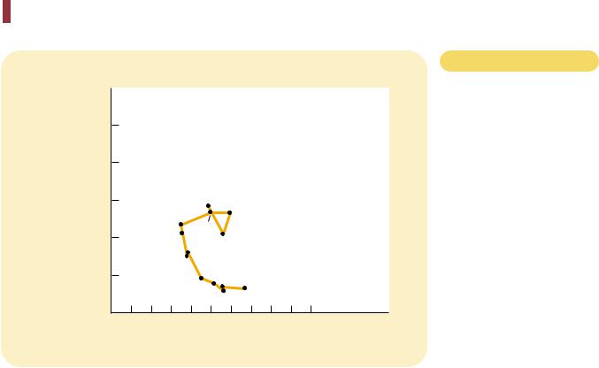


 inflation
780 |
PART TWELVE SHORT-RUN ECONOMIC FLUCTUATIONS |
to argue that when economic policies change, people adjust their expectations of inflation accordingly. Studies of inflation and unemployment that tried to estimate the sacrifice ratio had failed to take account of the direct effect of the policy regime on expectations. As a result, estimates of the sacrifice ratio were, according to the rational-expectations theorists, unreliable guides for policy.
In a 1981 paper titled “The End of Four Big Inflations,” Thomas Sargent described this new view as follows:
An alternative “rational expectations” view denies that there is any inherent momentum to the present process of inflation. This view maintains that firms and workers have now come to expect high rates of inflation in the future and that they strike inflationary bargains in light of these expectations. However, it is held that people expect high rates of inflation in the future precisely because the government’s current and prospective monetary and fiscal policies warrant those expectations. . . . An implication of this view is that inflation can be stopped much more quickly than advocates of the “momentum” view have indicated and that their estimates of the length of time and the costs of stopping inflation in terms of foregone output are erroneous. . . . This is not to say that it would be easy to eradicate inflation. On the contrary, it would require more than a few temporary restrictive fiscal and monetary actions. It would require a change in the policy regime. . . . How costly such a move would be in terms of foregone output and how long it would be in taking effect would depend partly on how resolute and evident the government’s commitment was.
According to Sargent, the sacrifice ratio could be much smaller than suggested by previous estimates. Indeed, in the most extreme case, it could be zero. If the government made a credible commitment to a policy of low inflation, people would be rational enough to lower their expectations of inflation immediately. The short-run Phillips curve would shift downward, and the economy would reach low inflation quickly without the cost of temporarily high unemployment and low output.
THE VOLCKER DISINFLATION
As we have seen, when Paul Volcker faced the prospect of reducing inflation from its peak of about 10 percent, the economics profession offered two conflicting predictions. One group of economists offered estimates of the sacrifice ratio and concluded that reducing inflation would have great cost in terms of lost output and high unemployment. Another group offered the theory of rational expectations and concluded that reducing inflation could be much less costly and, perhaps, could even have no cost at all. Who was right?
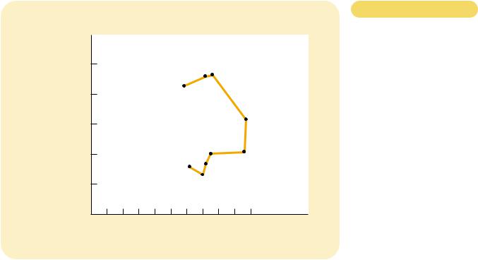
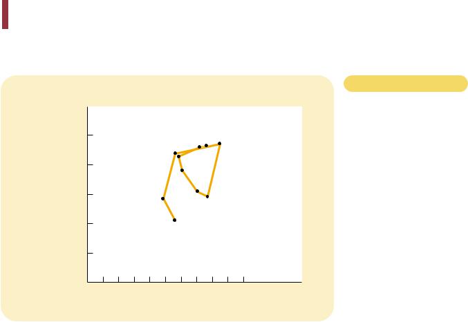
Figure 33-11 shows inflation and unemployment from 1979 to 1987. As you can see, Volcker did succeed at reducing inflation. Inflation came down from almost 10 percent in 1981 and 1982 to about 4 percent in 1983 and 1984. Credit for this reduction in inflation goes completely to monetary policy. Fiscal policy at this time was acting in the opposite direction: The increases in the budget deficit during the Reagan administration were expanding aggregate demand, which tends to raise inflation. The fall in inflation from 1981 to 1984 is attributable to the tough anti-inflation policies of Fed Chairman Paul Volcker.