Mankiw Principles of Economics (3rd ed)

QUICK QUIZ: Explain the three reasons why the aggregate-demand curve slopes downward. Give an example of an event that would shift the aggregate-demand curve. Which way would this event shift the curve?

THE AGGREGATE-SUPPLY CURVE

The aggregate-supply curve tells us the total quantity of goods and services that firms produce and sell at any given price level. Unlike the aggregate-demand curve, which is always downward sloping, the aggregate-supply curve shows a relationship that depends crucially on the time horizon being examined. In the long run, the aggregate-supply curve is vertical, whereas in the short run, the aggregate-supply curve is upward sloping. To understand short-run economic fluctuations, and how the short-run behavior of the economy deviates from its long-run behavior, we need to examine both the long-run aggregate-supply curve and the short-run aggregate-supply curve.

WHY THE AGGREGATE-SUPPLY CURVE

IS VERTICAL IN THE LONG RUN

What determines the quantity of goods and services supplied in the long run? We implicitly answered this question earlier in the book when we analyzed the process of economic growth. In the long run, an economy’s production of goods and services (its real GDP) depends on its supplies of labor, capital, and natural resources and on the available technology used to turn these factors of production into goods and services.

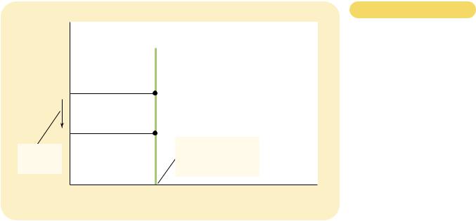
Because the price level does not affect these long-run determinants of real GDP, the long-run aggregate-supply curve is vertical, as in Figure 31-4. In other words, in the long run, the economy’s labor, capital, natural resources, and technology determine the total quantity of goods and services supplied, and this quantity supplied is the same regardless of what the price level happens to be.

The vertical long-run aggregate-supply curve is, in essence, just an application of the classical dichotomy and monetary neutrality. As we have already discussed, classical macroeconomic theory is based on the assumption that real variables do not depend on nominal variables. The long-run aggregate-supply curve is consistent with this idea because it implies that the quantity of output (a real variable) does not depend on the level of prices (a nominal variable). As noted earlier, most economists believe that this principle works well when studying the economy over a period of many years, but not when studying year-to-year changes. Thus, the aggregate-supply curve is vertical only in the long run.

One might wonder why supply curves for specific goods and services can be upward sloping if the long-run aggregate-supply curve is vertical. The reason is that the supply of specific goods and services depends on relative prices—the prices of those goods and services compared to other prices in the economy. For example, when the price of ice cream rises, suppliers of ice cream increase their production, taking labor, milk, chocolate, and other inputs away from the production of other goods, such as frozen yogurt. By contrast, the economy’s overall production of

the minimum wage substantially, the natural rate of unemployment would rise, and the economy would produce a smaller quantity of goods and services. As a result, the long-run aggregate-supply curve would shift to the left. Conversely, if a reform of the unemployment insurance system were to encourage unemployed workers to search harder for new jobs, the natural rate of unemployment would fall, and the long-run aggregate-supply curve would shift to the right.

Shifts Arising from Capital An increase in the economy’s capital stock increases productivity and, thereby, the quantity of goods and services supplied. As a result, the long-run aggregate-supply curve shifts to the right. Conversely, a decrease in the economy’s capital stock decreases productivity and the quantity of goods and services supplied, shifting the long-run aggregate-supply curve to the left.

Notice that the same logic applies regardless of whether we are discussing physical capital or human capital. An increase either in the number of machines or in the number of college degrees will raise the economy’s ability to produce goods and services. Thus, either would shift the long-run aggregate-supply curve to the right.

Shifts Arising from Natural Resources An economy’s production depends on its natural resources, including its land, minerals, and weather. A discovery of a new mineral deposit shifts the long-run aggregate-supply curve to the right. A change in weather patterns that makes farming more difficult shifts the long-run aggregate-supply curve to the left.

In many countries, important natural resources are imported from abroad. A change in the availability of these resources can also shift the aggregate-supply curve. As we discuss later in this chapter, events occurring in the world oil market have historically been an important source of shifts in aggregate supply.

Shifts Arising from Technological Knowledge Perhaps the most important reason that the economy today produces more than it did a generation ago is that our technological knowledge has advanced. The invention of the computer, for instance, has allowed us to produce more goods and services from any given amounts of labor, capital, and natural resources. As a result, it has shifted the long-run aggregate-supply curve to the right.

Although not literally technological, there are many other events that act like changes in technology. As Chapter 9 explains, opening up international trade has effects similar to inventing new production processes, so it also shifts the longrun aggregate-supply curve to the right. Conversely, if the government passed new regulations preventing firms from using some production methods, perhaps because they were too dangerous for workers, the result would be a leftward shift in the long-run aggregate-supply curve.

Summar y The long-run aggregate-supply curve reflects the classical model of the economy we developed in previous chapters. Any policy or event that raised real GDP in previous chapters can now be viewed as increasing the quantity of goods and services supplied and shifting the long-run aggregate-supply curve to the right. Any policy or event that lowered real GDP in previous chapters can now

The Misperceptions Theor y One approach to the short-run aggregatesupply curve is the misperceptions theory. According to this theory, changes in the overall price level can temporarily mislead suppliers about what is happening in the individual markets in which they sell their output. As a result of these shortrun misperceptions, suppliers respond to changes in the level of prices, and this response leads to an upward-sloping aggregate-supply curve.

To see how this might work, suppose the overall price level falls below the level that people expected. When suppliers see the prices of their products fall, they may mistakenly believe that their relative prices have fallen. For example, wheat farmers may notice a fall in the price of wheat before they notice a fall in the prices of the many items they buy as consumers. They may infer from this observation that the reward to producing wheat is temporarily low, and they may respond by reducing the quantity of wheat they supply. Similarly, workers may notice a fall in their nominal wages before they notice a fall in the prices of the goods they buy. They may infer that the reward to working is temporarily low and respond by reducing the quantity of labor they supply. In both cases, a lower price level causes misperceptions about relative prices, and these misperceptions induce suppliers to respond to the lower price level by decreasing the quantity of goods and services supplied.

The Sticky - Wage Theor y A second explanation of the upward slope of the short-run aggregate-supply curve is the sticky-wage theory. According to this theory, the short-run aggregate-supply curve slopes upward because nominal wages are slow to adjust, or are “sticky,” in the short run. To some extent, the slow adjustment of nominal wages is attributable to long-term contracts between workers and firms that fix nominal wages, sometimes for as long as three years. In addition, this slow adjustment may be attributable to social norms and notions of fairness that influence wage setting and that change only slowly over time.

To see what sticky nominal wages mean for aggregate supply, imagine that a firm has agreed in advance to pay its workers a certain nominal wage based on what it expected the price level to be. If the price level P falls below the level that was expected and the nominal wage remains stuck at W, then the real wage W/P rises above the level the firm planned to pay. Because wages are a large part of a firm’s production costs, a higher real wage means that the firm’s real costs have risen. The firm responds to these higher costs by hiring less labor and producing a smaller quantity of goods and services. In other words, because wages do not adjust immediately to the price level, a lower price level makes employment and production less profitable, which induces firms to reduce the quantity of goods and services supplied.

The Sticky - Price Theor y Recently, some economists have advocated a third approach to the short-run aggregate-supply curve, called the sticky-price theory. As we just discussed, the sticky-wage theory emphasizes that nominal wages adjust slowly over time. The sticky-price theory emphasizes that the prices of some goods and services also adjust sluggishly in response to changing economic conditions. This slow adjustment of prices occurs in part because there are costs to adjusting prices, called menu costs. These menu costs include the cost of printing and distributing catalogs and the time required to change price tags. As a result of these costs, prices as well as wages may be sticky in the short run.

To see the implications of sticky prices for aggregate supply, suppose that each firm in the economy announces its prices in advance based on the economic conditions it expects to prevail. Then, after prices are announced, the economy experiences an unexpected contraction in the money supply, which (as we have learned) will reduce the overall price level in the long run. Although some firms reduce their prices immediately in response to changing economic conditions, other firms may not want to incur additional menu costs and, therefore, may temporarily lag behind. Because these lagging firms have prices that are too high, their sales decline. Declining sales, in turn, cause these firms to cut back on production and employment. In other words, because not all prices adjust instantly to changing conditions, an unexpected fall in the price level leaves some firms with higher-than-desired prices, and these higher-than-desired prices depress sales and induce firms to reduce the quantity of goods and services they produce.

Summar y There are three alternative explanations for the upward slope of the short-run aggregate-supply curve: (1) misperceptions, (2) sticky wages, and (3) sticky prices. Economists debate which of these theories is correct. For our purposes in this book, however, the similarities of the theories are more important than the differences. All three theories suggest that output deviates from its natural rate when the price level deviates from the price level that people expected. We can express this mathematically as follows:

where a is a number that determines how much output responds to unexpected changes in the price level.

Notice that each of the three theories of short-run aggregate supply emphasizes a problem that is likely to be only temporary. Whether the upward slope of the aggregate-supply curve is attributable to misperceptions, sticky wages, or sticky prices, these conditions will not persist forever. Eventually, as people adjust their expectations, misperceptions are corrected, nominal wages adjust, and prices become unstuck. In other words, the expected and actual price levels are equal in the long run, and the aggregate-supply curve is vertical rather than upward sloping.

WHY THE SHORT-RUN AGGREGATE-SUPPLY

CURVE MIGHT SHIFT

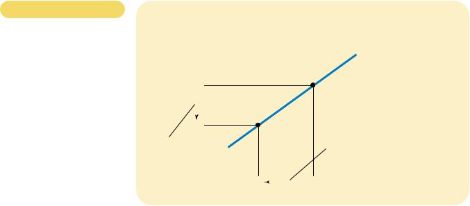
The short-run aggregate-supply curve tells us the quantity of goods and services supplied in the short run for any given level of prices. We can think of this curve as similar to the long-run aggregate-supply curve but made upward sloping by the presence of misperceptions, sticky wages, and sticky prices. Thus, when think-

ing about what shifts the short-run aggregate-supply curve, we have to consider all those variables that shift the long-run aggregate-supply curve plus a new variable—the expected price level—that influences misperceptions, sticky wages, and sticky prices.

Let’s start with what we know about the long-run aggregate-supply curve. As we discussed earlier, shifts in the long-run aggregate-supply curve normally arise from changes in labor, capital, natural resources, or technological knowledge. These same variables shift the short-run aggregate-supply curve. For example, when an increase in the economy’s capital stock increases productivity, both the long-run and short-run aggregate-supply curves shift to the right. When an increase in the minimum wage raises the natural rate of unemployment, both the long-run and short-run aggregate-supply curves shift to the left.

The important new variable that affects the position of the short-run aggregate-supply curve is people’s expectation of the price level. As we have discussed, the quantity of goods and services supplied depends, in the short run, on misperceptions, sticky wages, and sticky prices. Yet perceptions, wages, and prices are set on the basis of expectations of the price level. So when expectations change, the short-run aggregate-supply curve shifts.

To make this idea more concrete, let’s consider a specific theory of aggregate supply—the sticky-wage theory. According to this theory, when people expect the price level to be high, they tend to set wages high. High wages raise firms’ costs and, for any given actual price level, reduce the quantity of goods and services that firms supply. Thus, when the expected price level rises, wages rise, costs rise, and firms choose to supply a smaller quantity of goods and services at any given actual price level. Thus, the short-run aggregate-supply curve shifts to the left. Conversely, when the expected price level falls, wages fall, costs fall, firms increase production, and the short-run aggregate-supply curve shifts to the right.

A similar logic applies in each theory of aggregate supply. The general lesson is the following: An increase in the expected price level reduces the quantity of goods and services supplied and shifts the short-run aggregate-supply curve to the left. A decrease in the expected price level raises the quantity of goods and services supplied and shifts the short-run aggregate-supply curve to the right. As we will see in the next section, this influence of expectations on the position of the short-run aggregate-supply curve plays a key role in reconciling the economy’s behavior in the short run with its behavior in the long run. In the short run, expectations are fixed, and the economy finds itself at the intersection of the aggregate-demand curve and the short-run aggregate-supply curve. In the long run, expectations adjust, and the shortrun aggregate-supply curve shifts. This shift ensures that the economy eventually finds itself at the intersection of the aggregate-demand curve and the long-run aggregate-supply curve.

You should now have some understanding about why the short-run aggregate-supply curve slopes upward and what events and policies can cause this curve to shift. Table 31-2 summarizes our discussion.

QUICK QUIZ: Explain why the long-run aggregate-supply curve is vertical. Explain three theories for why the short-run aggregate-supply curve is upward sloping.