Mankiw Principles of Economics (3rd ed)
.pdf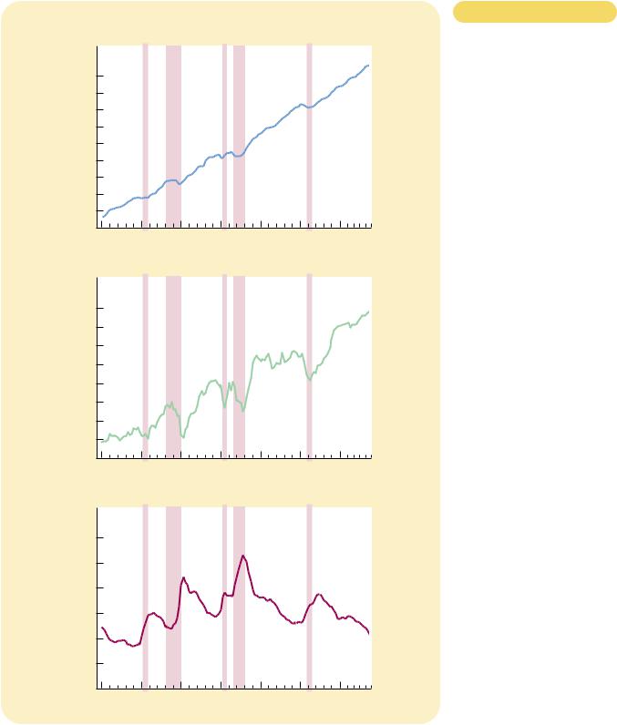


CHAPTER 31 AGGREGATE DEMAND AND AGGREGATE SUPPLY |
705 |
FACT 3: AS OUTPUT FALLS, UNEMPLOYMENT RISES
Changes in the economy’s output of goods and services are strongly correlated with changes in the economy’s utilization of its labor force. In other words, when real GDP declines, the rate of unemployment rises. This fact is hardly surprising: When firms choose to produce a smaller quantity of goods and services, they lay off workers, expanding the pool of unemployed.
Panel (c) of Figure 31-1 shows the unemployment rate in the U.S. economy since 1965. Once again, recessions are shown as the shaded areas in the figure. The figure shows clearly the impact of recessions on unemployment. In each of the recessions, the unemployment rate rises substantially. When the recession ends and real GDP starts to expand, the unemployment rate gradually declines. The unemployment rate never approaches zero; instead, it fluctuates around its natural rate of about 5 percent.
QUICK QUIZ: List and discuss three key facts about economic fluctuations.
EXPLAINING SHORT-RUN
ECONOMIC FLUCTUATIONS
Describing the regular patterns that economies experience as they fluctuate over time is easy. Explaining what causes these fluctuations is more difficult. Indeed, compared to the topics we have studied in previous chapters, the theory of economic fluctuations remains controversial. In this and the next two chapters, we develop the model that most economists use to explain short-run fluctuations in economic activity.
HOW THE SHORT RUN DIFFERS FROM THE LONG RUN
In previous chapters we developed theories to explain what determines most important macroeconomic variables in the long run. Chapter 24 explained the level and growth of productivity and real GDP. Chapter 25 explained how the real interest rate adjusts to balance saving and investment. Chapter 26 explained why there is always some unemployment in the economy. Chapters 27 and 28 explained the monetary system and how changes in the money supply affect the price level, the inflation rate, and the nominal interest rate. Chapters 29 and 30 extended this analysis to open economies in order to explain the trade balance and the exchange rate.
All of this previous analysis was based on two related ideas—the classical dichotomy and monetary neutrality. Recall that the classical dichotomy is the separation of variables into real variables (those that measure quantities or relative prices) and nominal variables (those measured in terms of money). According to classical macroeconomic theory, changes in the money supply affect nominal variables but not real variables. As a result of this monetary neutrality, Chapters 24, 25,


CHAPTER 31 AGGREGATE DEMAND AND AGGREGATE SUPPLY |
709 |
interest rates. Lower interest rates, in turn, encourage borrowing by firms that want to invest in new plants and equipment and by households who want to invest in new housing. Thus, a lower price level reduces the interest rate, encourages greater spending on investment goods, and thereby increases the quantity of goods and services demanded.
The Price Level and Net Expor ts: The Exchange - Rate Ef - fect As we have just discussed, a lower price level in the United States lowers the U.S. interest rate. In response, some U.S. investors will seek higher returns by investing abroad. For instance, as the interest rate on U.S. government bonds falls, a mutual fund might sell U.S. government bonds in order to buy German government bonds. As the mutual fund tries to move assets overseas, it increases the supply of dollars in the market for foreign-currency exchange. The increased supply of dollars causes the dollar to depreciate relative to other currencies. Because each dollar buys fewer units of foreign currencies, foreign goods become more expensive relative to domestic goods. This change in the real exchange rate (the relative price of domestic and foreign goods) increases U.S. exports of goods and services and decreases U.S. imports of goods and services. Net exports, which equal exports minus imports, also increase. Thus, when a fall in the U.S. price level causes U.S. interest rates to fall, the real exchange rate depreciates, and this depreciation stimulates U.S. net exports and thereby increases the quantity of goods and services demanded.
Summar y There are, therefore, three distinct but related reasons why a fall in the price level increases the quantity of goods and services demanded: (1) Consumers feel wealthier, which stimulates the demand for consumption goods. (2) Interest rates fall, which stimulates the demand for investment goods. (3) The exchange rate depreciates, which stimulates the demand for net exports. For all three reasons, the aggregate-demand curve slopes downward.
It is important to keep in mind that the aggregate-demand curve (like all demand curves) is drawn holding “other things equal.” In particular, our three explanations of the downward-sloping aggregate-demand curve assume that the money supply is fixed. That is, we have been considering how a change in the price level affects the demand for goods and services, holding the amount of money in the economy constant. As we will see, a change in the quantity of money shifts the aggregate-demand curve. At this point, just keep in mind that the aggregate-demand curve is drawn for a given quantity of money.
WHY THE AGGREGATE-DEMAND CURVE MIGHT SHIFT
The downward slope of the aggregate-demand curve shows that a fall in the price level raises the overall quantity of goods and services demanded. Many other factors, however, affect the quantity of goods and services demanded at a given price level. When one of these other factors changes, the aggregate-demand curve shifts.
Let’s consider some examples of events that shift aggregate demand. We can categorize them according to which component of spending is most directly affected.
Shifts Arising from Consumption Suppose Americans suddenly become more concerned about saving for retirement and, as a result, reduce their current consumption. Because the quantity of goods and services demanded at
710 |
PART TWELVE SHORT-RUN ECONOMIC FLUCTUATIONS |
any price level is lower, the aggregate-demand curve shifts to the left. Conversely, imagine that a stock market boom makes people feel wealthy and less concerned about saving. The resulting increase in consumer spending means a greater quantity of goods and services demanded at any given price level, so the aggregatedemand curve shifts to the right.
Thus, any event that changes how much people want to consume at a given price level shifts the aggregate-demand curve. One policy variable that has this effect is the level of taxation. When the government cuts taxes, it encourages people to spend more, so the aggregate-demand curve shifts to the right. When the government raises taxes, people cut back on their spending, and the aggregatedemand curve shifts to the left.
Shifts Arising from Investment Any event that changes how much firms want to invest at a given price level also shifts the aggregate-demand curve. For instance, imagine that the computer industry introduces a faster line of computers, and many firms decide to invest in new computer systems. Because the quantity of goods and services demanded at any price level is higher, the aggregate-demand curve shifts to the right. Conversely, if firms become pessimistic about future business conditions, they may cut back on investment spending, shifting the aggregate-demand curve to the left.
Tax policy can also influence aggregate demand through investment. As we saw in Chapter 25, an investment tax credit (a tax rebate tied to a firm’s investment spending) increases the quantity of investment goods that firms demand at any given interest rate. It therefore shifts the aggregate-demand curve to the right. The repeal of an investment tax credit reduces investment and shifts the aggregatedemand curve to the left.
Another policy variable that can influence investment and aggregate demand is the money supply. As we discuss more fully in the next chapter, an increase in the money supply lowers the interest rate in the short run. This makes borrowing less costly, which stimulates investment spending and thereby shifts the aggregate-demand curve to the right. Conversely, a decrease in the money supply raises the interest rate, discourages investment spending, and thereby shifts the aggregate-demand curve to the left. Many economists believe that throughout U.S. history changes in monetary policy have been an important source of shifts in aggregate demand.
Shifts Arising from Government Purchases The most direct way that policymakers shift the aggregate-demand curve is through government purchases. For example, suppose Congress decides to reduce purchases of new weapons systems. Because the quantity of goods and services demanded at any price level is lower, the aggregate-demand curve shifts to the left. Conversely, if state governments start building more highways, the result is a greater quantity of goods and services demanded at any price level, so the aggregate-demand curve shifts to the right.
Shifts Arising from Net Expor ts Any event that changes net exports for a given price level also shifts aggregate demand. For instance, when Europe experiences a recession, it buys fewer goods from the United States. This reduces U.S. net exports and shifts the aggregate-demand curve for the U.S. economy to