628 |
PART TEN MONEY AND PRICES IN THE LONG RUN |
Accumulated over so many years, a 5 percent annual inflation rate leads to an 18-fold increase in the price level.
Inflation may seem natural and inevitable to a person who grew up in the United States during the second half of the twentieth century, but in fact it is not inevitable at all. There were long periods in the nineteenth century during which most prices fell—a phenomenon called deflation. The average level of prices in the U.S. economy was 23 percent lower in 1896 than in 1880, and this deflation was a major issue in the presidential election of 1896. Farmers, who had accumulated large debts, were suffering when the fall in crop prices reduced their incomes and thus their ability to pay off their debts. They advocated government policies to reverse the deflation.
Although inflation has been the norm in more recent history, there has been substantial variation in the rate at which prices rise. During the 1990s, prices rose at an average rate of about 2 percent per year. By contrast, in the 1970s, prices rose by 7 percent per year, which meant a doubling of the price level over the decade. The public often views such high rates of inflation as a major economic problem. In fact, when President Jimmy Carter ran for reelection in 1980, challenger Ronald Reagan pointed to high inflation as one of the failures of Carter’s economic policy.
International data show an even broader range of inflation experiences. Germany after World War I experienced a spectacular example of inflation. The price of a newspaper rose from 0.3 marks in January 1921 to 70,000,000 marks less than two years later. Other prices rose by similar amounts. An extraordinarily high rate of inflation such as this is called hyperinflation. The German hyperinflation had such an adverse effect on the German economy that it is often viewed as one contributor to the rise of Nazism and, as a result, World War II. Over the past 50 years, with this episode still in mind, German policymakers have been extraordinarily averse to inflation, and Germany has had much lower inflation than the United States.
What determines whether an economy experiences inflation and, if so, how much? This chapter answers this question by developing the quantity theory of money. Chapter 1 summarized this theory as one of the Ten Principles of Economics: Prices rise when the government prints too much money. This insight has a long and venerable tradition among economists. The quantity theory was discussed by the famous eighteenth-century philosopher David Hume and has been advocated more recently by the prominent economist Milton Friedman. This theory of inflation can explain both moderate inflations, such as those we have experienced in the United States, and hyperinflations, such as those experienced in interwar Germany and, more recently, in some Latin American countries.
After developing a theory of inflation, we turn to a related question: Why is inflation a problem? At first glance, the answer to this question may seem obvious: Inflation is a problem because people don’t like it. In the 1970s, when the United States experienced a relatively high rate of inflation, opinion polls placed inflation as the most important issue facing the nation. President Ford echoed this sentiment in 1974 when he called inflation “public enemy number one.” Ford briefly wore a “WIN” button on his lapel—for “Whip Inflation Now.”
But what, exactly, are the costs that inflation imposes on a society? The answer may surprise you. Identifying the various costs of inflation is not as straightforward as it first appears. As a result, although all economists decry hyperinflation, some economists argue that the costs of moderate inflation are not nearly as large as the general public believes.
CHAPTER 28 MONEY GROWTH AND INFLATION |
629 |
THE CLASSICAL THEORY OF INFLATION
We begin our study of inflation by developing the quantity theory of money. This theory is often called “classical” because it was developed by some of the earliest thinkers about economic issues. Most economists today rely on this theory to explain the long-run determinants of the price level and the inflation rate.
THE LEVEL OF PRICES AND THE VALUE OF MONEY
Suppose we observe over some period of time the price of an ice-cream cone rising from a nickel to a dollar. What conclusion should we draw from the fact that people are willing to give up so much more money in exchange for a cone? It is possible that people have come to enjoy ice cream more (perhaps because some chemist has developed a miraculous new flavor). Yet that is probably not the case. It is more likely that people’s enjoyment of ice cream has stayed roughly the same and that, over time, the money used to buy ice cream has become less valuable. Indeed, the first insight about inflation is that it is more about the value of money than about the value of goods.
This insight helps point the way toward a theory of inflation. When the consumer price index and other measures of the price level rise, commentators are often tempted to look at the many individual prices that make up these price indexes: “The CPI rose by 3 percent last month, led by a 20 percent rise in the price of coffee and a 30 percent rise in the price of heating oil.” Although this approach does contain some interesting information about what’s happening in the
”So what’s it going to be? The same size as last year or the same price as last year?”
630 |
PART TEN MONEY AND PRICES IN THE LONG RUN |
economy, it also misses a key point: Inflation is an economy-wide phenomenon that concerns, first and foremost, the value of the economy’s medium of exchange.
The economy’s overall price level can be viewed in two ways. So far, we have viewed the price level as the price of a basket of goods and services. When the price level rises, people have to pay more for the goods and services they buy. Alternatively, we can view the price level as a measure of the value of money. A rise in the price level means a lower value of money because each dollar in your wallet now buys a smaller quantity of goods and services.
It may help to express these ideas mathematically. Suppose P is the price level as measured, for instance, by the consumer price index or the GDP deflator. Then P measures the number of dollars needed to buy a basket of goods and services. Now turn this idea around: The quantity of goods and services that can be bought with $1 equals 1/P. In other words, if P is the price of goods and services measured in terms of money, 1/P is the value of money measured in terms of goods and services. Thus, when the overall price level rises, the value of money falls.
MONEY SUPPLY, MONEY DEMAND,
AND MONETARY EQUILIBRIUM
What determines the value of money? The answer to this question, like many in economics, is supply and demand. Just as the supply and demand for bananas determines the price of bananas, the supply and demand for money determines the value of money. Thus, our next step in developing the quantity theory of money is to consider the determinants of money supply and money demand.
First consider money supply. In the preceding chapter we discussed how the Federal Reserve, together with the banking system, determines the supply of money. When the Fed sells bonds in open-market operations, it receives dollars in exchange and contracts the money supply. When the Fed buys government bonds, it pays out dollars and expands the money supply. In addition, if any of these dollars are deposited in banks who then hold them as reserves, the money multiplier swings into action, and these open-market operations can have an even greater effect on the money supply. For our purposes in this chapter, we ignore the complications introduced by the banking system and simply take the quantity of money supplied as a policy variable that the Fed controls directly and completely.
Now consider money demand. There are many factors that determine the quantity of money people demand, just as there are many determinants of the quantity demanded of other goods and services. How much money people choose to hold in their wallets, for instance, depends on how much they rely on credit cards and on whether an automatic teller machine is easy to find. And, as we will emphasize in Chapter 32, the quantity of money demanded depends on the interest rate that a person could earn by using the money to buy an interest-bearing bond rather than leaving it in a wallet or low-interest checking account.
Although many variables affect the demand for money, one variable stands out in importance: the average level of prices in the economy. People hold money because it is the medium of exchange. Unlike other assets, such as bonds or stocks, people can use money to buy the goods and services on their shopping lists. How much money they choose to hold for this purpose depends on the prices of those goods and services. The higher prices are, the more money the typical transaction requires, and the more money people will choose to hold in their wallets and
632 |
PART TEN MONEY AND PRICES IN THE LONG RUN |
THE EFFECTS OF A MONETARY INJECTION
quantity theor y of money a theory asserting that the quantity of money available determines the price level and that the growth rate in the quantity of money available determines the inflation rate
Figur e 28-2
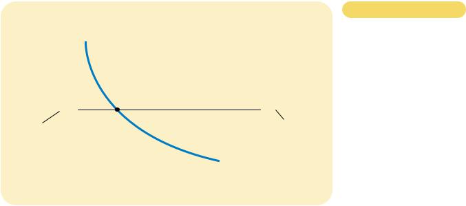
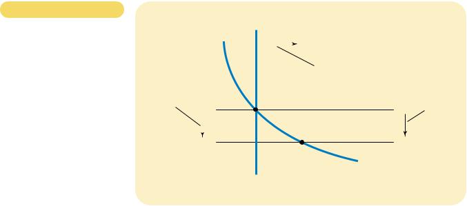
AN INCREASE IN THE
MONEY SUPPLY. When the Fed increases the supply of money, the money supply curve shifts from MS1 to MS2. The value of money (on the left axis) and the price level (on the right axis) adjust to bring supply and demand back into balance. The equilibrium moves from point A to point B. Thus, when an increase in the money supply makes dollars more plentiful, the
price level increases, making each dollar less valuable.
Let’s now consider the effects of a change in monetary policy. To do so, imagine that the economy is in equilibrium and then, suddenly, the Fed doubles the supply of money by printing some dollar bills and dropping them around the country from helicopters. (Or, less dramatically and more realistically, the Fed could inject money into the economy by buying some government bonds from the public in open-market operations.) What happens after such a monetary injection? How does the new equilibrium compare to the old one?
Figure 28-2 shows what happens. The monetary injection shifts the supply curve to the right from MS1 to MS2, and the equilibrium moves from point A to point B. As a result, the value of money (shown on the left axis) decreases from 1/2 to 1/4, and the equilibrium price level (shown on the right axis) increases from 2 to 4. In other words, when an increase in the money supply makes dollars more plentiful, the result is an increase in the price level that makes each dollar less valuable.
This explanation of how the price level is determined and why it might change over time is called the quantity theory of money. According to the quantity theory, the quantity of money available in the economy determines the value of money, and growth in the quantity of money is the primary cause of inflation. As economist Milton Friedman once put it, “Inflation is always and everywhere a monetary phenomenon.”
A BRIEF LOOK AT THE ADJUSTMENT PROCESS
So far we have compared the old equilibrium and the new equilibrium after an injection of money. How does the economy get from the old to the new equilibrium?
Value of |
|
MS1 |
MS2 |
|
|
|
Price |
Money, 1/P |
|
|
|
|
Level, P |
(High) 1 |
|
|
|
|
|
|
|
|
|
1 |
(Low) |
|
|
|
|
|
|
|
|
|
|
|
|
|
|
|
|
|
|
|
|
|
|
|
|
|
|
|
|
|
1. An increase |
|
|
|
|
|
3/4 |
|
|
|
|
|
in the money |
|
|
|
1.33 |
|
|
|
|
|
|
|
2. …decreases |
|
|
|
|
|
|
|
|
|
|
|
|
|
supply... |
|
|
|
|
|
|
the value of |
|
|
|
|
|
|
|
|
|
|
|
|
|
|
|
|
|
|
|
|
|
|
|
|
|
|
|
3. …and |
money… |
|
|
|
A |
|
|
|
|
|
|
|
|
1/2 |
|
|
|
|
|
|
|
2 |
|
increases |
|
|
|
|
|
|
|
|
|
|
|
|
|
|
|
|
|
|
|
|
|
|
|
|
|
|
|
|
|
|
|
|
|
|
the price |
|
|
|
|
|
|
|
|
|
|
|
|
|
|
|
|
|
|
|
|
|
|
|
|
|
|
|
level. |
|
|
|
|
|
|
|
B |
|
|
|
4 |
|
|
1/4 |
|
|
|
|
|
|
|
|
|
|
|
|
|
|
|
|
|
|
|
|
|
|
|
|
|
|
Money |
|
|
|
|
|
|
|
|
|
|
|
|
|
|
|
|
|
|
|
|
|
|
|
demand |
|
|
|
(Low) |
|
|
|
|
|
|
|
|
|
|
(High) |
0 |
|
M1 |
M2 |
Quantity of |
|
|
636 |
PART TEN MONEY AND PRICES IN THE LONG RUN |
Figur e 28-3
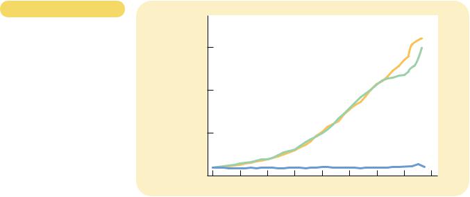
NOMINAL GDP, THE
QUANTITY OF MONEY, AND
THE VELOCITY OF MONEY. This
figure shows the nominal value of output as measured by nominal GDP, the quantity of money as measured by M2, and the velocity of money as measured by their ratio. For comparability, all three series have been scaled to equal 100 in 1960. Notice that nominal GDP and the quantity of money have grown dramatically over this period, while velocity has been relatively stable.
Indexes |
|
|
|
|
|
|
|
|
(1960 = 100) |
|
|
|
|
|
|
|
|
1,500 |
|
|
|
|
|
|
|
|
|
|
|
|
|
Nominal GDP |
|
1,000 |
|
|
|
|
|
|
M2 |
|
|
|
|
|
|
|
|
|
500 |
|
|
|
|
|
|
|
|
|
|
|
|
|
|
Velocity |
|
|
0 |
1965 |
1970 |
1975 |
1980 |
1985 |
1990 |
1995 |
2000 |
1960 |
SOURCE: U.S. Department of Commerce;
Federal Reserve Board.
The price level must rise, the quantity of output must rise, or the velocity of money must fall.
In many cases, it turns out that the velocity of money is relatively stable. For example, Figure 28-3 shows nominal GDP, the quantity of money (as measured by M2), and the velocity of money for the U.S. economy since 1960. Although the velocity of money is not exactly constant, it has not changed dramatically. By contrast, the money supply and nominal GDP during this period have increased more than tenfold. Thus, for some purposes, the assumption of constant velocity may be a good approximation.
We now have all the elements necessary to explain the equilibrium price level and inflation rate. Here they are:
1.The velocity of money is relatively stable over time.
2.Because velocity is stable, when the Fed changes the quantity of money (M), it causes proportionate changes in the nominal value of output (P Y).
3.The economy’s output of goods and services (Y) is primarily determined by factor supplies (labor, physical capital, human capital, and natural resources) and the available production technology. In particular, because money is neutral, money does not affect output.
4.With output (Y) determined by factor supplies and technology, when the Fed alters the money supply (M) and induces proportional changes in the nominal value of output (P Y), these changes are reflected in changes in the price level (P).
5.Therefore, when the Fed increases the money supply rapidly, the result is a high rate of inflation.
These five steps are the essence of the quantity theory of money.
CHAPTER 28 MONEY GROWTH AND INFLATION |
637 |
(a) Austria
Index |
|
|
|
|
(Jan. 1921 = 100) |
|
|
|
|
100,000 |
|
|
|
|
10,000 |
Price level |
|
|
|
|
Money supply |
|
|
|
|
1,000 |
|
|
|
|
100 |
1922 |
1923 |
1924 |
1925 |
1921 |
(b) Hungary
Index |
|
|
|
|
(July 1921 = 100) |
|
|
|
|
100,000 |
|
|
|
|
|
|
Price level |
|
10,000 |
|
|
|
|
1,000 |
|
|
Money supply |
|
|
|
|
100 |
1922 |
1923 |
1924 |
1925 |
1921 |
Index |
|
|
|
|
Index |
|
|
|
|
(Jan. 1921 = 100) |
|
|
|
|
(Jan. 1921 = 100) |
|
|
|
|
100,000,000,000,000 |
|
Price level |
|
10,000,000 |
|
|
|
|
1,000,000,000,000 |
|
|
1,000,000 |
|
Price level |
|
|
|
Money |
|
|
10,000,000,000 |
|
|
|
|
|
|
|
|
|
|
|
|
|
supply |
100,000 |
|
|
Money |
100,000,000 |
|
|
|
|
1,000,000 |
|
|
|
|
10,000 |
|
|
supply |
|
|
|
|
|
|
|
|
|
10,000 |
|
|
|
|
1,000 |
|
|
|
|
100 |
|
|
|
|
|
|
|
|
|
|
|
|
|
|
|
|
|
1 |
1922 |
1923 |
1924 |
1925 |
100 |
1922 |
1923 |
1924 |
1925 |
1921 |
1921 |
|
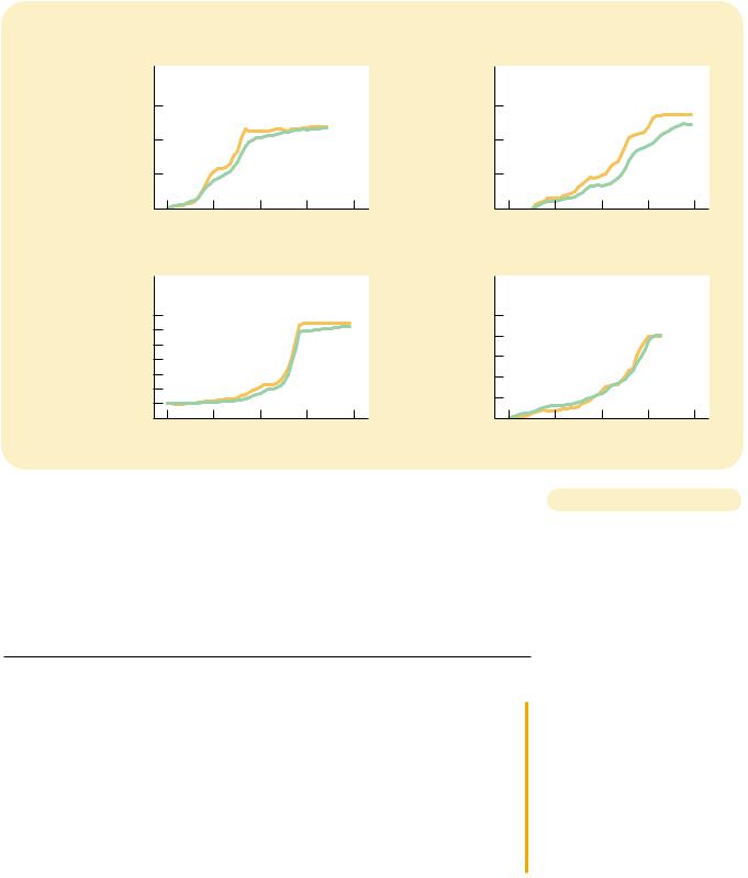
MONEY AND PRICES DURING FOUR HYPERINFLATIONS. This figure shows the quantity |
Figur e 28-4 |
|
of money and the price level during four hyperinflations. (Note that these variables are |
|
|
|
graphed on logarithmic scales. This means that equal vertical distances on the graph |
|
|
represent equal percentage changes in the variable.) In each case, the quantity of money |
|
|
and the price level move closely together. The strong association between these two |
|
|
variables is consistent with the quantity theory of money, which states that growth in |
|
|
the money supply is the primary cause of inflation. |
|
SOURCE: Adapted from Thomas J. Sargent, “The End of Four Big Inflations,” in Robert Hall, ed., Inflation, Chicago:
University of Chicago Press, 1983, pp. 41-93.
CASE STUDY MONEY AND PRICES DURING
FOUR HYPERINFLATIONS
Although earthquakes can wreak havoc on a society, they have the beneficial by-product of providing much useful data for seismologists. These data can shed light on alternative theories and, thereby, help society predict and deal with future threats. Similarly, hyperinflations offer monetary economists a natural experiment they can use to study the effects of money on the economy.
Hyperinflations are interesting in part because the changes in the money supply and price level are so large. Indeed, hyperinflation is generally defined