568 |
PART NINE THE REAL ECONOMY IN THE LONG RUN |
POLICY 1: TAXES AND SAVING
American families save a smaller fraction of their incomes than their counterparts in many other countries, such as Japan and Germany. Although the reasons for these international differences are unclear, many U.S. policymakers view the low level of U.S. saving as a major problem. One of the Ten Principles of Economics in Chapter 1 is that a country’s standard of living depends on its ability to produce goods and services. And, as we discussed in the preceding chapter, saving is an important long-run determinant of a nation’s productivity. If the United States could somehow raise its saving rate to the level that prevails in other countries, the growth rate of GDP would increase, and over time, U.S. citizens would enjoy a higher standard of living.
Another of the Ten Principles of Economics is that people respond to incentives. Many economists have used this principle to suggest that the low saving rate in the United States is at least partly attributable to tax laws that discourage saving. The U.S. federal government, as well as many state governments, collects revenue by taxing income, including interest and dividend income. To see the effects of this policy, consider a 25-year-old individual who saves $1,000 and buys a 30-year bond that pays an interest rate of 9 percent. In the absence of taxes, the $1,000 grows to $13,268 when the individual reaches age 55. Yet if that interest is taxed at a rate of, say, 33 percent, then the after-tax interest rate is only 6 percent. In this case, the $1,000 grows to only $5,743 after 30 years. The tax on interest income substantially reduces the future payoff from current saving and, as a result, reduces the incentive for people to save.
In response to this problem, many economists and lawmakers have proposed changing the tax code to encourage greater saving. In 1995, for instance, when Congressman Bill Archer of Texas became chairman of the powerful House Ways and Means Committee, he proposed replacing the current income tax with a consumption tax. Under a consumption tax, income that is saved would not be taxed until the saving is later spent; in essence, a consumption tax is like the sales taxes that many states now use to collect revenue. A more modest proposal is to expand eligibility for special accounts, such as Individual Retirement Accounts, that allow people to shelter some of their saving from taxation. Let’s consider the effect of such a saving incentive on the market for loanable funds, as illustrated in Figure 25-2.
First, which curve would this policy affect? Because the tax change would alter the incentive for households to save at any given interest rate, it would affect the quantity of loanable funds supplied at each interest rate. Thus, the supply of loanable funds would shift. The demand for loanable funds would remain the same, because the tax change would not directly affect the amount that borrowers want to borrow at any given interest rate.
Second, which way would the supply curve shift? Because saving would be taxed less heavily than under current law, households would increase their saving by consuming a smaller fraction of their income. Households would use this additional saving to increase their deposits in banks or to buy more bonds. The supply of loanable funds would increase, and the supply curve would shift to the right from S1 to S2, as shown in Figure 25-2.
Finally, we can compare the old and new equilibria. In the figure, the increased supply of loanable funds reduces the interest rate from 5 percent to 4 percent. The lower interest rate raises the quantity of loanable funds demanded from $1,200
CHAPTER 25 SAVING, INVESTMENT, AND THE FINANCIAL SYSTEM |
569 |
Figur e 25-2
5%
4%
2. ...which reduces the equilibrium interest rate...
3. ...and raises the equilibrium quantity of loanable funds.
S2
1. Tax incentives for saving increase the supply of loanable funds...
Demand
Loanable Funds (in billions of dollars)
AN INCREASE IN THE SUPPLY OF LOANABLE FUNDS. A change
in the tax laws to encourage Americans to save more would shift the supply of loanable funds to the right from S1 to S2. As a result, the equilibrium interest rate would fall, and the lower interest rate would stimulate investment. Here the equilibrium interest rate falls from 5 percent to 4 percent, and the equilibrium quantity of loanable funds saved and invested rises from $1,200 billion to $1,600 billion.
billion to $1,600 billion. That is, the shift in the supply curve moves the market equilibrium along the demand curve. With a lower cost of borrowing, households and firms are motivated to borrow more to finance greater investment. Thus, if a change in the tax laws encouraged greater saving, the result would be lower interest rates and greater investment.
Although this analysis of the effects of increased saving is widely accepted among economists, there is less consensus about what kinds of tax changes should be enacted. Many economists endorse tax reform aimed at increasing saving in order to stimulate investment and growth. Yet others are skeptical that these tax changes would have much effect on national saving. These skeptics also doubt the equity of the proposed reforms. They argue that, in many cases, the benefits of the tax changes would accrue primarily to the wealthy, who are least in need of tax relief. We examine this debate more fully in the final chapter of this book.
POLICY 2: TAXES AND INVESTMENT
Suppose that Congress passed a law giving a tax reduction to any firm building a new factory. In essence, this is what Congress does when it institutes an investment tax credit, which it does from time to time. Let’s consider the effect of such a law on the market for loanable funds, as illustrated in Figure 25-3.
First, would the law affect supply or demand? Because the tax credit would reward firms that borrow and invest in new capital, it would alter investment at any given interest rate and, thereby, change the demand for loanable funds. By contrast, because the tax credit would not affect the amount that households save at any given interest rate, it would not affect the supply of loanable funds.
570 |
PART NINE THE REAL ECONOMY IN THE LONG RUN |
Figur e 25-3
AN INCREASE IN THE DEMAND
FOR LOANABLE FUNDS. If the
passage of an investment tax credit encouraged U.S. firms to invest more, the demand for loanable funds would increase. As a result, the equilibrium interest rate would rise, and the higher interest rate would
stimulate saving. Here, when the demand curve shifts from D1 to D2, the equilibrium interest rate rises from 5 percent to 6 percent, and the equilibrium quantity
of loanable funds saved and invested rises from $1,200 billion to $1,400 billion.
Interest
|
Rate |
Supply |
|
|
1. An investment |
|
|
|
|
|
|
|
|
|
|
|
|
tax credit |
|
6% |
|
|
increases the |
|
|
|
demand for |
|
|
|
|
|
|
|
|
|
|
|
|
|
5% |
|
|
loanable funds... |
|
|
|
|
|
|
|
2. ...which |
|
|
|
|
|
|
|
|
|
|
|
|
raises the |
|
|
|
|
D2 |
|
equilibrium |
|
|
Demand, D1 |
|
interest rate... |
|
|
|
|
|
|
|
|
|
0 |
$1,200 |
|
$1,400 |
Loanable Funds |
|
(in billions of dollars)
3. ...and raises the equilibrium quantity of loanable funds.
Second, which way would the demand curve shift? Because firms would have an incentive to increase investment at any interest rate, the quantity of loanable funds demanded would be higher at any given interest rate. Thus, the demand curve for loanable funds would move to the right, as shown by the shift from D1 to D2 in the figure.
Third, consider how the equilibrium would change. In Figure 25-3, the increased demand for loanable funds raises the interest rate from 5 percent to 6 percent, and the higher interest rate in turn increases the quantity of loanable funds supplied from $1,200 billion to $1,400 billion, as households respond by increasing the amount they save. This change in household behavior is represented here as a movement along the supply curve. Thus, if a change in the tax laws encouraged greater investment, the result would be higher interest rates and greater saving.
POLICY 3:
GOVERNMENT BUDGET DEFICITS AND SURPLUSES
Throughout the 1980s and 1990s, one of the most pressing policy issues was the size of the government budget deficit. Recall that a budget deficit is an excess of government spending over tax revenue. Governments finance budget deficits by borrowing in the bond market, and the accumulation of past government borrowing is called the government debt. In the 1980s and 1990s, the U.S. federal government ran large budget deficits, resulting in a rapidly growing government debt. As a result, much public debate centered on the effects of these deficits both on the allocation of the economy’s scarce resources and on long-term economic growth.
572 |
PART NINE THE REAL ECONOMY IN THE LONG RUN |
Thus, the most basic lesson about budget deficits follows directly from their effects on the supply and demand for loanable funds: When the government reduces national saving by running a budget deficit, the interest rate rises, and investment falls.
Because investment is important for long-run economic growth, government budget deficits reduce the economy’s growth rate.
Government budget surpluses work just the opposite as budget deficits. When government collects more in tax revenue than it spends, its saves the difference by retiring some of the outstanding government debt. This budget surplus, or public saving, contributes to national saving. Thus, a budget surplus increases the supply of loanable funds, reduces the interest rate, and stimulates investment. Higher investment, in turn, means greater capital accumulation and more rapid economic growth.
CASE STUDY THE DEBATE OVER THE BUDGET SURPLUS
Our analysis shows why, other things being the same, budget surpluses are better for economic growth than budget deficits. Making economic policy, however, is not as simple as this observation may make it sound. A good example occurred in the late 1990s, when the U.S. government found itself with a budget surplus, and much debate centered on what to do with it.
Many policymakers favored leaving the budget surplus alone, rather than dissipating it with a spending increase or tax cut. They based their conclusion on the analysis we have just seen: Using the surplus to retire some of the government debt would stimulate private investment and economic growth.
Other policymakers took a different view. Some thought the surplus should be used to increase government spending on infrastructure and education because, they argued, the return to these public investments is greater than the typical return to private investment. Some thought taxes should be cut, arguing that lower tax rates would distort decisionmaking less and lead to a more efficient allocation of resources; they also cautioned that without such a tax cut,
“Our debt-reduction plan is simple, but it will require a great deal of money.”
CHAPTER 25 SAVING, INVESTMENT, AND THE FINANCIAL SYSTEM |
573 |
Congress would be tempted to spend the surplus on “pork barrel” projects of dubious value.
As this book was going to press, the debate over the budget surplus was still raging. There is room for reasonable people to disagree. The right policy depends on how valuable you view private investment, how valuable you view public investment, how distortionary you view taxation, and how reliable you view the political process.
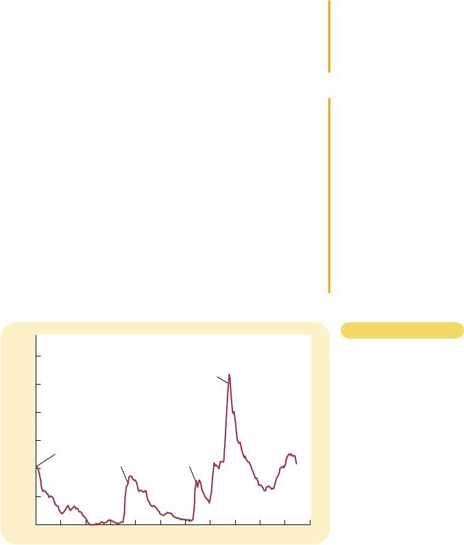
CASE STUDY THE HISTORY OF U.S. GOVERNMENT DEBT
How indebted is the U.S. government? The answer to this question varies substantially over time. Figure 25-5 shows the debt of the U.S. federal government expressed as a percentage of U.S. GDP. It shows that the government debt has fluctuated from zero in 1836 to 107 percent of GDP in 1945. In recent years, government debt has been about 50 percent of GDP.
The behavior of the debt–GDP ratio is one gauge of what’s happening with the government’s finances. Because GDP is a rough measure of the government’s tax base, a declining debt–GDP ratio indicates that the government indebtedness is shrinking relative to its ability to raise tax revenue. This suggests that the government is, in some sense, living within its means. By contrast, a rising debt–GDP ratio means that the government indebtedness is increasing relative to its ability to raise tax revenue. It is often interpreted as meaning that fiscal policy—government spending and taxes—cannot be sustained forever at current levels.
Throughout history, the primary cause of fluctuations in government debt is war. When wars occur, government spending on national defense rises
Percent
of GDP
120
World War II
100
80
60
Revolutionary |
|
|
War |
Civil |
World War I |
|
War |
40
20
0 |
1810 |
1830 |
1850 |
1870 |
1890 |
1910 |
1930 |
1950 |
1970 |
1990 |
2010 |
1790 |
Figur e 25-5
THE U.S. GOVERNMENT DEBT.
The debt of the U.S. federal government, expressed here as a percentage of GDP, has varied substantially throughout history. It reached its highest level after the large expenditures of World
War II, but then declined throughout the 1950s and 1960s. It began rising again in the early 1980s when Ronald Reagan’s tax cuts were not accompanied by similar cuts in government spending.
It then stabilized and even declined slightly in the late 1990s.
Source: U.S. Department of Treasury; U.S. Department of Commerce; and T. S. Berry, “Production and Population since 1789,” Bostwick Paper No. 6, Richmond, 1988.
574 |
PART NINE THE REAL ECONOMY IN THE LONG RUN |
substantially to pay for soldiers and military equipment. Taxes typically rise as well but by much less than the increase in spending. The result is a budget deficit and increasing government debt. When the war is over, government spending declines, and the debt–GDP ratio starts declining as well.
There are two reasons to believe that debt financing of war is an appropriate policy. First, it allows the government to keep tax rates smooth over time. Without debt financing, tax rates would have to rise sharply during wars, and as we saw in Chapter 8, this would cause a substantial decline in economic efficiency. Second, debt financing of wars shifts part of the cost of wars to future generations, who will have to pay off the government debt. This is arguably a fair distribution of the burden, for future generations get some of the benefit when one generation fights a war to defend the nation against foreign aggressors.
One large increase in government debt that cannot be explained by war is the increase that occurred beginning around 1980. When President Ronald Reagan took office in 1981, he was committed to smaller government and lower taxes. Yet he found cutting government spending to be more difficult politically than cutting taxes. The result was the beginning of a period of large budget deficits that continued not only through Reagan’s time in office but also for many years thereafter. As a result, government debt rose from 26 percent of GDP in 1980 to 50 percent of GDP in 1993.
As we discussed earlier, government budget deficits reduce national saving, investment, and long-run economic growth, and this is precisely why the rise in government debt during the 1980s troubled so many economists. Policymakers from both political parties accepted this basic argument and viewed persistent budget deficits as an important policy problem. When Bill Clinton moved into the Oval Office in 1993, deficit reduction was his first major goal. Similarly, when the Republicans took control of Congress in 1995, deficit reduction was high on their legislative agenda. Both of these efforts substantially reduced the size of the government budget deficit, and it eventually turned into a small surplus. As a result, by the late 1990s, the debt–GDP ratio was declining once again.
QUICK QUIZ: If more Americans adopted a “live for today” approach to life, how would this affect saving, investment, and the interest rate?
CONCLUSION
“Neither a borrower nor a lender be,” Polonius advises his son in Shakespeare’s Hamlet. If everyone followed this advice, this chapter would have been unnecessary.
Few economists would agree with Polonius. In our economy, people borrow and lend often, and usually for good reason. You may borrow one day to start your own business or to buy a home. And people may lend to you in the hope that the interest you pay will allow them to enjoy a more prosperous retirement. The financial system has the job of coordinating all this borrowing and lending activity.

CHAPTER 25 SAVING, INVESTMENT, AND THE FINANCIAL SYSTEM |
575 |
In many ways, financial markets are like other markets in the economy. The price of loanable funds—the interest rate—is governed by the forces of supply and demand, just as other prices in the economy are. And we can analyze shifts in supply or demand in financial markets as we do in other markets. One of the Ten Principles of Economics introduced in Chapter 1 is that markets are usually a good way to organize economic activity. This principle applies to financial markets as well. When financial markets bring the supply and demand for loanable funds into balance, they help allocate the economy’s scarce resources to their most efficient use.
In one way, however, financial markets are special. Financial markets, unlike most other markets, serve the important role of linking the present and the future. Those who supply loanable funds—savers—do so because they want to convert some of their current income into future purchasing power. Those who demand loanable funds—borrowers—do so because they want to invest today in order to have additional capital in the future to produce goods and services. Thus, wellfunctioning financial markets are important not only for current generations but also for future generations who will inherit many of the resulting benefits.
Summar y
The U.S. financial system is made financial institutions, such as the market, banks, and mutual funds act to direct the resources of save some of their income into and firms who want to borrow.
National income accounting important relationships among variables. In particular, for a saving must equal investment. the mechanism through which one person’s saving with another
The interest rate is determined demand for loanable funds. The
households who want to save some lend it out. The demand for
from households and firms who investment. To analyze how any
the interest rate, one must the supply and demand for
private saving plus public budget deficit represents negative
therefore, reduces national saving loanable funds available to finance
government budget deficit crowds reduces the growth of productivity
Key Concepts
financial system, p. 554 financial markets, p. 555 bond, p. 555
stock, p. 556
financial intermediaries, p. 556
budget deficit, p. 562
market for loanable funds, p. 564 crowding out, p. 571
1.What is the role of the financial system? Name and describe two markets that are part of the financial
system in our economy. Name and describe two financial intermediaries.