CHAPTER 23 MEASURING THE COST OF LIVING |
517 |
|
|
|
|
names) price-taker Mary Ann Latter squints at a sale sign above an ivory shell blouse. “Save 45%–60% when you take an additional 30% off permanently reduced merchandise. Markdown taken at register,” the sign says.
Confused, Ms. Latter asks a clerk to scan the item. There is a pause. “It’s 30 percent off,” she says, just before the lunch-hour rush.
“I know,” Ms. Latter says, “but can you scan it just to make sure?” Under her breath, she mumbles, “So helpful.” Downstairs in the jewelry department, Ms. Latter tries to price the one 18-inch silver necklace left, but there is no tag. “Do I have to look it up now?” moans the employee behind the counter. Ms. Latter watches her wait on several customers, then asks again: “Could you find it?” The harried saleswoman throws on the counter a thick notebook with a dizzying array of jewelry sketches. Ms. Latter finally locates a silver weave that
looks about right.
When the exact item can’t be found, price-takers must substitute. That can be difficult. Consider a haircut: If the stylist leaves, his fill-in must have about the same experience; a newer stylist, for example, might charge less. This frigid
winter afternoon, Ms. Latter needs to substitute a coat because clothing items rarely remain on the racks for more than a couple months. It must be a lightweight swing coat of less than half wool. After digging through heavy winter wear, trying to locate tags in three departments on two floors, she gives up. It is off season anyway, so she will have to wait months to choose a substitute.
Making it harder for price detectives to grasp the true cost of living is that the master list of 207 categories they price—called the market basket—is updated only once every ten years. Cellular phones? Too new to be priced because they don’t fit into any of the categories set up in the 1980s. They probably will be included when the new categories arrive [next year].
Some changes within these categories are made every five years. So within “new cars,” for example, if domestic autos overtake imports in a big way, price-takers might examine more Fords and fewer Toyotas. But that doesn’t happen often enough, critics say. Ms. Latter, a city-dwelling Generation X’er, continually must price “Always Twenty-One” girdles, yet ignore the new, popular WonderBras behind her. . . .
Ms. Latter’s colleague in suburban Chicago, Sheila Ward, must ignore the hoopla over Tickle Me Elmo and instead price a GI Joe Extreme doll with “painted, molded hair.” Reliance on outdated goods, says Mrs. Ward, “would be one of the criticisms of us.” She recalls a music store owner who became frustrated because she kept seeking prices on a guitar he could never imagine playing— much less selling. He finally threw her out of his shop, screaming, “The damned government! Is this what I’m paying taxes for?”
Price-takers can’t do much about these problems. What they can do is interrogate. At a simple restaurant, Mrs. Ward asks if food portions have changed. The owner says they haven’t. But she remembers that the price of bacon has been climbing, and asks again about his BLT. Suddenly, he recalls that he has cut the number of bacon slices from three to two. And that is a very different sandwich.
SOURCE: The Wall Street Journal, January 16, 1997, p. A1.
to include VCRs, and subsequently the index reflected changes in VCR prices. But the reduction in the cost of living associated with the initial introduction of the VCR never showed up in the index.
The third problem with the consumer price index is unmeasured quality change. If the quality of a good deteriorates from one year to the next, the value of a dollar falls, even if the price of the good stays the same. Similarly, if the quality rises from one year to the next, the value of a dollar rises. The Bureau of Labor Statistics does its best to account for quality change. When the quality of a good in the basket changes—for example, when a car model has more horsepower or gets better gas mileage from one year to the next—the BLS adjusts the price of the good to account for the quality change. It is, in essence, trying to compute the price of a basket of goods of constant quality. Despite these efforts, changes in quality remain a problem, because quality is so hard to measure.
518 |
PART EIGHT THE DATA OF MACROECONOMICS |
There is still much debate among economists about how severe these measurement problems are and what should be done about them. The issue is important because many government programs use the consumer price index to adjust for changes in the overall level of prices. Recipients of Social Security, for instance, get annual increases in benefits that are tied to the consumer price index. Some economists have suggested modifying these programs to correct for the measurement problems. For example, most studies conclude that the consumer price index overstates inflation by about 1 percentage point per year (although recent improvements in the CPI have reduced this upward bias somewhat). In response to these findings, Congress could change the Social Security program so that benefits increased every year by the measured inflation rate minus 1 percentage point. Such a change would provide a crude way of offsetting the measurement problems and, at the same time, reduce government spending by billions of dollars each year.
|
|
|
ndex “is understating |
|
|
|
|
IN THE NEWS |
|
n for the elderly,” |
|
|
n economist at the |
|
|
|
|
A CPI for Senior Citizens |
|
nstitute, |
an indepen- |
|
|
|
nization in Washing- |
|
|
|
is likely to |
get |
|
|
|
the |
author |
of |
|
|
|
Right: The Battle Over |
|
|
|
Index,” said older |
|
|
1.3 percent next year. But the costs that |
people’s higher spending on some |
|
|
drain the resources of many retired |
goods and services was not the only |
|
|
people—notably medical treatment, pre- |
reason. The official index also considers |
|
|
scription drugs, and special housing— |
price declines for consumer goods that |
|
|
are rising faster than consumer prices in |
they rarely buy, like television sets and |
|
|
general. . . . |
computers. |
|
|
|
|
Now the Bureau of Labor Statistics, |
While Congress balks at the cost, |
|
|
which calculates the indexes, has |
he added, a separate CPI for the elderly |
|
|
devised an experimental index that does |
“would be the way to go” to correct the |
|
|
track some spending habits of older |
problem. |
|
|
|
|
Americans, and it has shown a widening |
|
|
|
|
|
gap between cost increases for them |
SOURCE: The New York Times, Business Section, |
|
|
|
and those for the general population. |
November 8, 1998, p. 10. |
|
|
|
R e t i r e e s ’ R e a l i t y ? |
Between December 1982 and Septem- |
|
|
|
|
|
ber 1998, the experimental index rose |
|
|
|
|
BY LAURA CASTANEDA |
73.9 percent, while the official index |
|
|
|
|
Low inflation, a driving force behind the |
rose 63.5 percent, said Patrick Jack- |
|
|
|
|
nation’s economic boom, is having the |
man, an economist at the bureau. . . . |
|
|
|
|
|
|
|
|
|
|
|
|
|
|
|
CHAPTER 23 MEASURING THE COST OF LIVING |
519 |
THE GDP DEFLATOR VERSUS THE CONSUMER PRICE INDEX
In the preceding chapter, we examined another measure of the overall level of prices in the economy—the GDP deflator. The GDP deflator is the ratio of nominal GDP to real GDP. Because nominal GDP is current output valued at current prices and real GDP is current output valued at base-year prices, the GDP deflator reflects the current level of prices relative to the level of prices in the base year.
Economists and policymakers monitor both the GDP deflator and the consumer price index to gauge how quickly prices are rising. Usually, these two statistics tell a similar story. Yet there are two important differences that can cause them to diverge.
The first difference is that the GDP deflator reflects the prices of all goods and services produced domestically, whereas the consumer price index reflects the prices of all goods and services bought by consumers. For example, suppose that the price of an airplane produced by Boeing and sold to the Air Force rises. Even though the plane is part of GDP, it is not part of the basket of goods and services bought by a typical consumer. Thus, the price increase shows up in the GDP deflator but not in the consumer price index.
As another example, suppose that Volvo raises the price of its cars. Because Volvos are made in Sweden, the car is not part of U.S. GDP. But U.S. consumers buy Volvos, and so the car is part of the typical consumer’s basket of goods. Hence, a price increase in an imported consumption good, such as a Volvo, shows up in the consumer price index but not in the GDP deflator.
This first difference between the consumer price index and the GDP deflator is particularly important when the price of oil changes. Although the United States does produce some oil, much of the oil we use is imported from the Middle East. As a result, oil and oil products such as gasoline and heating oil comprise a much larger share of consumer spending than they do of GDP. When the price of oil rises, the consumer price index rises by much more than does the GDP deflator.
The second and more subtle difference between the GDP deflator and the consumer price index concerns how various prices are weighted to yield a single number for the overall level of prices. The consumer price index compares the price of a fixed basket of goods and services to the price of the basket in the base year. Only occasionally does the Bureau of Labor Statistics change the basket of goods. By contrast, the GDP deflator compares the price of currently produced goods and services to the price of the same goods and services in the base year. Thus, the group of goods and services used to compute the GDP deflator changes automatically over time. This difference is not important when all prices are changing proportionately. But if the prices of different goods and services are changing by varying amounts, the way we weight the various prices matters for the overall inflation rate.
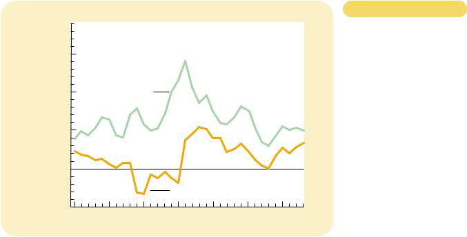
Figure 23-2 shows the inflation rate as measured by both the GDP deflator and the consumer price index for each year since 1965. You can see that sometimes the two measures diverge. When they do diverge, it is possible to go behind these numbers and explain the divergence with the two differences we have discussed. The figure shows, however, that divergence between these two measures is the exception rather than the rule. In the late 1970s, both the GDP deflator and the consumer price index show high rates of inflation. In the late 1980s and 1990s, both measures show low rates of inflation.
520 |
PART EIGHT THE DATA OF MACROECONOMICS |
Figure 23-2
TWO MEASURES OF INFLATION.
This figure shows the inflation rate—the percentage change in the level of prices—as measured by the GDP deflator and the consumer price index using annual data since 1965. Notice that the two measures of inflation generally move together.
SOURCE: U.S. Department of Labor; U.S.
Department of Commerce.
Percent per Year
15
CPI
10
0 |
1970 |
1975 |
1980 |
1985 |
1990 |
1995 1998 |
1965 |
QUICK QUIZ: Explain briefly what the consumer price index is trying to measure and how it is constructed.
|
|
CORRECTING ECONOMIC VARIABLES FOR THE |
|
|
EFFECTS OF INFLATION |
|
|
|
|
|
|
|
The purpose of measuring the overall level of prices in the economy is to permit |
|
|
comparison between dollar figures from different points in time. Now that we |
|
|
know how price indexes are calculated, let’s see how we might use such an index |
|
|
to compare a dollar figure from the past to a dollar figure in the present. |
|
|
DOLLAR FIGURES FROM DIFFERENT TIMES |
|
|
We first return to the issue of Babe Ruth’s salary. Was his salary of $80,000 in 1931 |
|
|
high or low compared to the salaries of today’s players? |
|
|
To answer this question, we need to know the level of prices in 1931 and the |
|
|
level of prices today. Part of the increase in baseball salaries just compensates play- |
|
|
”The price may seem a little high, |
ers for the higher level of prices today. To compare Ruth’s salary to those of today’s |
but you have to remember that’s |
players, we need to inflate Ruth’s salary to turn 1931 dollars into today’s dollars. |
in today’s dollars.” |
A price index determines the size of this inflation correction. |

CHAPTER 23 MEASURING THE COST OF LIVING |
521 |
Government statistics show a consumer price index of 15.2 for 1931 and 166 for 1999. Thus, the overall level of prices has risen by a factor of 10.9 (which equals 166/15.2). We can use these numbers to measure Ruth’s salary in 1999 dollars. The calculation is as follows:
Salary in 1999 dollars Salary in 1931 dollars
Price level in 1999
Price level in 1931
166$80,000 15.2
$873,684.
We find that Babe Ruth’s 1931 salary is equivalent to a salary today of just under $1 million. That is not a bad income, but it is less than the salary of the average baseball player today, and it is far less than the amount paid to today’s baseball superstars. Chicago Cubs hitter Sammy Sosa, for instance, was paid about $10 million in 1999.
Let’s also examine President Hoover’s 1931 salary of $75,000. To translate that figure into 1999 dollars, we again multiply the ratio of the price levels in the two years. We find that Hoover’s salary is equivalent to $75,000 (166/15.2), or $819,079, in 1999 dollars. This is well above President Clinton’s salary of $200,000 (and even above the $400,000 salary that, according to recent legislation, will be paid to Clinton’s successor). It seems that President Hoover did have a pretty good year after all.
CASE STUDY MR. INDEX GOES TO HOLLYWOOD
What was the most popular movie of all time? The answer might surprise you. Movie popularity is usually gauged by box office receipts. By that measure, Titanic is the No. 1 movie of all time, followed by Star Wars, Star Wars: The Phantom Menace, and ET. But this ranking ignores an obvious but important fact: Prices, including the price of movie tickets, have been rising over time. When we correct box office receipts for the effects of inflation, the story is very
different.
Table 23-2 shows the top ten movies of all time, ranked by inflationadjusted box office receipts. The No. 1 movie is Gone with the Wind, which was released in 1939 and is well ahead of Titanic. In the 1930s, before everyone had televisions in their homes, about 90 million Americans went to the cinema each week, compared to about 25 million today. But the movies from that era rarely show up in popularity rankings because ticket prices were only a quarter. Scarlett and Rhett fare a lot better once we correct for the effects of inflation.
INDEXATION
“FRANKLY, MY DEAR, I DON’T CARE MUCH
FOR THE EFFECTS OF INFLATION.”
As we have just seen, price indexes are used to correct for the effects of inflation |
|
when comparing dollar figures from different times. This type of correction shows |
indexation |
up in many places in the economy. When some dollar amount is automatically |
the automatic correction of a dollar |
corrected for inflation by law or contract, the amount is said to be indexed for |
amount for the effects of inflation |
inflation. |
by law or contract |