482 |
PART SEVEN ADVANCED TOPIC |
consumption rises. Yet the response of leisure to the change in the wage is different in the two cases. In panel (a), Sally responds to the higher wage by enjoying less leisure. In panel (b), Sally responds by enjoying more leisure.
Sally’s decision between leisure and consumption determines her supply of labor, for the more leisure she enjoys the less time she has left to work. In each panel, the right-hand graph in Figure 21-14 shows the labor supply curve implied by Sally’s decision. In panel (a), a higher wage induces Sally to enjoy less leisure and work more, so the labor supply curve slopes upward. In panel (b), a higher wage induces Sally to enjoy more leisure and work less, so the labor supply curve slopes “backward.”
At first, the backward-sloping labor supply curve is puzzling. Why would a person respond to a higher wage by working less? The answer comes from considering the income and substitution effects of a higher wage.
Consider first the substitution effect. When Sally’s wage rises, leisure becomes more costly relative to consumption, and this encourages Sally to substitute consumption for leisure. In other words, the substitution effect induces Sally to work harder in response to higher wages, which tends to make the labor supply curve slope upward.
Now consider the income effect. When Sally’s wage rises, she moves to a higher indifference curve. She is now better off than she was. As long as consumption and leisure are both normal goods, she tends to want to use this increase in well-being to enjoy both higher consumption and greater leisure. In other words, the income effect induces her to work less, which tends to make the labor supply curve slope backward.
In the end, economic theory does not give a clear prediction about whether an increase in the wage induces Sally to work more or less. If the substitution effect is greater than the income effect for Sally, she works more. If the income effect is greater than the substitution effect, she works less. The labor supply curve, therefore, could be either upward or backward sloping.
CASE STUDY INCOME EFFECTS ON LABOR SUPPLY: HISTORICAL TRENDS, LOTTERY WINNERS, AND THE CARNEGIE CONJECTURE
The idea of a backward-sloping labor supply curve might at first seem like a mere theoretical curiosity, but in fact it is not. Evidence indicates that the labor supply curve, considered over long periods of time, does in fact slope backward. A hundred years ago many people worked six days a week. Today five-day workweeks are the norm. At the same time that the length of the workweek has been falling, the wage of the typical worker (adjusted for inflation) has been rising.
Here is how economists explain this historical pattern: Over time, advances in technology raise workers’ productivity and, thereby, the demand for labor. The increase in labor demand raises equilibrium wages. As wages rise, so does the reward for working. Yet rather than responding to this increased incentive by working more, most workers choose to take part of their greater prosperity in the form of more leisure. In other words, the income effect of higher wages dominates the substitution effect.
Further evidence that the income effect on labor supply is strong comes from a very different kind of data: winners of lotteries. Winners of large prizes
CHAPTER 21 THE THEORY OF CONSUMER CHOICE |
483 |
in the lottery see large increases in their incomes and, as a result, large outward shifts in their budget constraints. Because the winners’ wages have not changed, however, the slopes of their budget constraints remain the same. There is, therefore, no substitution effect. By examining the behavior of lottery winners, we can isolate the income effect on labor supply.
The results from studies of lottery winners are striking. Of those winners who win more than $50,000, almost 25 percent quit working within a year, and another 9 percent reduce the number of hours they work. Of those winners who win more than $1 million, almost 40 percent stop working. The income effect on labor supply of winning such a large prize is substantial.
Similar results were found in a study, published in the May 1993 issue of the Quarterly Journal of Economics, of how receiving a bequest affects a person’s labor supply. The study found that a single person who inherits more than $150,000 is four times as likely to stop working as a single person who inherits less than $25,000. This finding would not have surprised the nineteenth-century industrialist Andrew Carnegie. Carnegie warned that “the parent who leaves his son enormous wealth generally deadens the talents and energies of the son, and tempts him to lead a less useful and less worthy life than he otherwise would.” That is, Carnegie viewed the income effect on labor supply to be substantial and, from his paternalistic perspective, regrettable. During his life and at his death, Carnegie gave much of his vast fortune to charity.
HOW DO INTEREST RATES AFFECT HOUSEHOLD SAVING?
An important decision that every person faces is how much income to consume today and how much to save for the future. We can use the theory of consumer choice to analyze how people make this decision and how the amount they save depends on the interest rate their savings will earn.
Consider the decision facing Sam, a worker planning ahead for retirement. To keep things simple, let’s divide Sam’s life into two periods. In the first period, Sam is young and working. In the second period, he is old and retired. When young, Sam earns a total of $100,000. He divides this income between current consumption and saving. When he is old, Sam will consume what he has saved, including the interest that his savings have earned.
Suppose that the interest rate is 10 percent. Then for every dollar that Sam saves when young, he can consume $1.10 when old. We can view “consumption when young” and “consumption when old” as the two goods that Sam must choose between. The interest rate determines the relative price of these two goods.
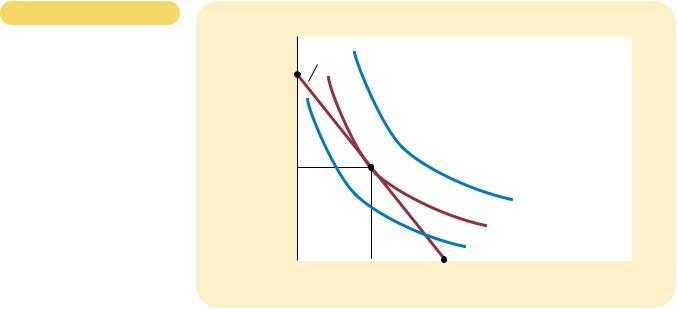
Figure 21-15 shows Sam’s budget constraint. If he saves nothing, he consumes $100,000 when young and nothing when old. If he saves everything, he consumes nothing when young and $110,000 when old. The budget constraint shows these and all the intermediate possibilities.
Figure 21-15 uses indifference curves to represent Sam’s preferences for consumption in the two periods. Because Sam prefers more consumption in both periods, he prefers points on higher indifference curves to points on lower ones. Given his preferences, Sam chooses the optimal combination of consumption in both periods of life, which is the point on the budget constraint that is on the highest possible indifference curve. At this optimum, Sam consumes $50,000 when young and $55,000 when old.
484 |
PART SEVEN ADVANCED TOPIC |
Figur e 21-15
THE CONSUMPTION-SAVING
DECISION. This figure shows the budget constraint for a person deciding how much to consume in the two periods of his life, the indifference curves representing his preferences, and the optimum.
Consumption Budget
when Old constraint
$110,000
55,000 |
Optimum |
|
|
|
|
|
I 3 |
|
|
|
I 2 |
|
|
|
I 1 |
0 |
$50,000 |
100,000 |
Consumption |
|
|
|
when Young |
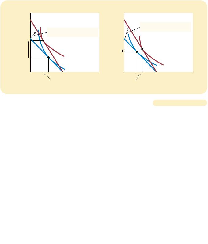
Now consider what happens when the interest rate increases from 10 percent to 20 percent. Figure 21-16 shows two possible outcomes. In both cases, the budget constraint shifts outward and becomes steeper. At the new higher interest rate, Sam gets more consumption when old for every dollar of consumption that he gives up when young.
The two panels show different preferences for Sam and the resulting response to the higher interest rate. In both cases, consumption when old rises. Yet the response of consumption when young to the change in the interest rate is different in the two cases. In panel (a), Sam responds to the higher interest rate by consuming less when young. In panel (b), Sam responds by consuming more when young.
Sam’s saving, of course, is his income when young minus the amount he consumes when young. In panel (a), consumption when young falls when the interest rate rises, so saving must rise. In panel (b), Sam consumes more when young, so saving must fall.
The case shown in panel (b) might at first seem odd: Sam responds to an increase in the return to saving by saving less. Yet this behavior is not as peculiar as it might seem. We can understand it by considering the income and substitution effects of a higher interest rate.
Consider first the substitution effect. When the interest rate rises, consumption when old becomes less costly relative to consumption when young. Therefore, the substitution effect induces Sam to consume more when old and less when young. In other words, the substitution effect induces Sam to save more.
Now consider the income effect. When the interest rate rises, Sam moves to a higher indifference curve. He is now better off than he was. As long as consumption in both periods consists of normal goods, he tends to want to use this increase in well-being to enjoy higher consumption in both periods. In other words, the income effect induces him to save less.
|
|
CHAPTER 21 |
|
(a) Higher Interest Rate Raises Saving |
|
Consumption |
|
Consumption |
when Old |
BC2 |
when Old |
1. A higher interest rate rotates the budget constraint outward . . .
BC1
I 2
I 1
THE THEORY OF CONSUMER CHOICE |
485 |
(b) Higher Interest Rate Lowers Saving
BC2
1. A higher interest rate rotates the budget constraint outward . . .
BC1
I 1 I 2
0 |
|
|
|
Consumption |
0 |
|
|
|
Consumption |
|
|
|
|
|
|
|
2. . . . resulting in lower |
when Young |
|
2. . . . resulting in higher |
when Young |
|
|
|
|
|
consumption when young |
|
|
consumption when young |
|
|
and, thus, higher saving. |
|
|
and, thus, lower saving. |
|
|
|
|
|
|
|
|
|
|
|
|
AN INCREASE IN THE INTEREST RATE. In both panels, an increase in the interest rate |
Figur e 21-16 |
|
shifts the budget constraint outward. In panel (a), consumption when young falls, and |
|
|
|
consumption when old rises. The result is an increase in saving when young. In panel (b), |
|
|
consumption in both periods rises. The result is a decrease in saving when young. |
|
|
|
|
|
The end result, of course, depends on both the income and substitution effects. If the substitution effect of a higher interest rate is greater than the income effect, Sam saves more. If the income effect is greater than the substitution effect, Sam saves less. Thus, the theory of consumer choice says that an increase in the interest rate could either encourage or discourage saving.
Although this ambiguous result is interesting from the standpoint of economic theory, it is disappointing from the standpoint of economic policy. It turns out that an important issue in tax policy hinges in part on how saving responds to interest rates. Some economists have advocated reducing the taxation of interest and other capital income, arguing that such a policy change would raise the after-tax interest rate that savers can earn and would thereby encourage people to save more. Other economists have argued that because of offsetting income and substitution effects, such a tax change might not increase saving and could even reduce it. Unfortunately, research has not led to a consensus about how interest rates affect saving. As a result, there remains disagreement among economists about whether changes in tax policy aimed to encourage saving would, in fact, have the intended effect.
DO THE POOR PREFER TO RECEIVE CASH
OR IN-KIND TRANSFERS?
Paul is a pauper. Because of his low income, he has a meager standard of living. The government wants to help. It can either give Paul $1,000 worth of food
486 |
PART SEVEN |
ADVANCED TOPIC |
|
|
|
|
|
|
|
|
|
|
(a) The Constraint Is Not Binding |
|
|
|
|
|
Cash Transfer |
|
|
In-Kind Transfer |
|
|
Food |
|
|
|
Food |
|
|
|
|
|
BC2 (with $1,000 cash) |
|
BC2 (with $1,000 food stamps) |
|
|
|
|
|
|
|
|
|
BC1 |
|
|
BC1 |
|
|
|
|
|
B |
|
|
B |
|
|
$1,000 |
|
|
I2 |
$1,000 |
|
|
|
I2 |
|
|
|
A |
|
|
A |
|
|
|
|
|
|
|
|
|
|
|
|
|
|
|
|
|
|
|
|
|
|
|
I1 |
|
|
I1 |
|
|
|
|
|
|
|
|
|
|
|
|
|
|
|
0 |
|
|
Nonfood |
0 |
|
|
|
|
Nonfood |
|
|
|
|
Consumption |
|
|
|
|
|
Consumption |
|
|
|
|
(b) The Constraint Is Binding |
|
|
|
|
|
Cash Transfer |
|
|
In-Kind Transfer |
|
|
Food |
|
|
|
Food |
|
|
|
|
|
|
|
BC2 (with $1,000 cash) |
|
BC2 (with $1,000 food stamps) |
|
|
|
|
|
|
|
|
|
BC1 |
|
|
BC1 |
|
|
$1,000 |
|
|
B |
$1,000 |
|
A |
|
B |
|
|
|
|
|
|
|
|
|
|
|
|
|
|
|
|
|
|
|
A |
|
|
|
|
|
|
|
|
|
I2 |
|
|
|
|
I1 |
I2 |
|
|
|
|
I1 |
|
|
|
|
I3 |
|
0 |
|
|
Nonfood |
0 |
|
|
|
|
Nonfood |
|
|
|
|
Consumption |
|
|
|
|
|
Consumption |
Figur e 21-17
CASH VERSUS IN-KIND TRANSFERS. Both panels compare a cash transfer and a similar in-kind transfer of food. In panel (a), the in-kind transfer does not impose a binding constraint, and the consumer ends up on the same indifference curve under the two policies. In panel (b), the in-kind transfer imposes a binding constraint, and the consumer ends up on a lower indifference curve with the in-kind transfer than with the cash transfer.
(perhaps by issuing him food stamps) or simply give him $1,000 in cash. What does the theory of consumer choice have to say about the comparison between these two policy options?
Figure 21-17 shows how the two options might work. If the government gives Paul cash, then the budget constraint shifts outward. He can divide the extra cash
CHAPTER 21 THE THEORY OF CONSUMER CHOICE |
487 |
between food and nonfood consumption however he pleases. By contrast, if the government gives Paul an in-kind transfer of food, then his new budget constraint is more complicated. The budget constraint has again shifted out. But now the budget constraint has a kink at $1,000 of food, for Paul must consume at least that amount in food. That is, even if Paul spends all his money on nonfood consumption, he still consumes $1,000 in food.
The ultimate comparison between the cash transfer and in-kind transfer depends on Paul’s preferences. In panel (a), Paul would choose to spend at least $1,000 on food even if he receives a cash transfer. Therefore, the constraint imposed by the in-kind transfer is not binding. In this case, his consumption moves from point A to point B regardless of the type of transfer. That is, Paul’s choice between food and nonfood consumption is the same under the two policies.
In panel (b), however, the story is very different. In this case, Paul would prefer to spend less than $1,000 on food and spend more on nonfood consumption. The cash transfer allows him discretion to spend the money as he pleases, and he consumes at point B. By contrast, the in-kind transfer imposes the binding constraint that he consume at least $1,000 of food. His optimal allocation is at the kink, point C. Compared to the cash transfer, the in-kind transfer induces Paul to consume more food and less of other goods. The in-kind transfer also forces Paul to end up on a lower (and thus less preferred) indifference curve. Paul is worse off than if he had the cash transfer.
Thus, the theory of consumer choice teaches a simple lesson about cash versus in-kind transfers. If an in-kind transfer of a good forces the recipient to consume more of the good than he would on his own, then the recipient prefers the cash transfer. If the in-kind transfer does not force the recipient to consume more of the good than he would on his own, then the cash and in-kind transfer have exactly the same effect on the consumption and welfare of the recipient.
QUICK QUIZ: Explain how an increase in the wage can potentially decrease the amount that a person wants to work.
CONCLUSION: DO PEOPLE
REALLY THINK THIS WAY?
The theory of consumer choice describes how people make decisions. As we have seen, it has broad applicability. It can explain how a person chooses between Pepsi and pizza, work and leisure, consumption and saving, and on and on.
At this point, however, you might be tempted to treat the theory of consumer choice with some skepticism. After all, you are a consumer. You decide what to buy every time you walk into a store. And you know that you do not decide by writing down budget constraints and indifference curves. Doesn’t this knowledge about your own decisionmaking provide evidence against the theory?
The answer is no. The theory of consumer choice does not try to present a literal account of how people make decisions. It is a model. And, as we first discussed in Chapter 2, models are not intended to be completely realistic.
The best way to view the theory of consumer choice is as a metaphor for how consumers make decisions. No consumer (except an occasional economist) goes
488 |
PART SEVEN ADVANCED TOPIC |
through the explicit optimization envisioned in the theory. Yet consumers are aware that their choices are constrained by their financial resources. And, given those constraints, they do the best they can to achieve the highest level of satisfaction. The theory of consumer choice tries to describe this implicit, psychological process in a way that permits explicit, economic analysis.
The proof of the pudding is in the eating. And the test of a theory is in its applications. In the last section of this chapter we applied the theory of consumer choice to four practical issues about the economy. If you take more advanced courses in economics, you will see that this theory provides the framework for much additional analysis.
A consumer’s budget constraint combinations of different goods income and the prices of the goods budget constraint equals the
The consumer’s indifference preferences. An indifference curve bundles of goods that make the happy. Points on higher indifference preferred to points on lower
slope of an indifference curve at consumer’s marginal rate of which the consumer is willing to other.
The consumer optimizes by budget constraint that lies on the curve. At this point, the slope of (the marginal rate of substitution equals the slope of the budget price of the goods).
Summar y
good falls, the impact on the
can be broken down into an income effect. The income effect is the that arises because a lower price better off. The substitution effect is
consumption that arises because a price greater consumption of the good
relatively cheaper. The income effect is movement from a lower to a higher
whereas the substitution effect is along an indifference curve to
slope.
choice can be applied in many explain why demand curves can upward, why higher wages could decrease the quantity of labor
interest rates could either increase and why the poor prefer cash to
Key Concepts
budget constraint, p. 465 indifference curve, p. 466
marginal rate of substitution, p. 467 perfect substitutes, p. 470
substitution effect, p. 475 good, p. 479
1.A consumer has income of $3,000. Wine costs $3 a glass, and cheese costs $6 a pound. Draw the consumer’s
budget constraint. What is the slope of this budget constraint?
CHAPTER 21 THE THEORY OF CONSUMER CHOICE |
489 |
2.Draw a consumer’s indifference curves for wine and cheese. Describe and explain four properties of these indifference curves.
3.Pick a point on an indifference curve for wine and cheese and show the marginal rate of substitution. What does the marginal rate of substitution tell us?
4.Show a consumer’s budget constraint and indifference curves for wine and cheese. Show the optimal consumption choice. If the price of wine is $3 a glass and the price of cheese is $6 a pound, what is the marginal rate of substitution at this optimum?
5.A person who consumes wine and his income increases from $3,000 happens if both wine and cheese Now show what happens if cheese
6.The price of cheese rises from $6 to $10 a pound, while the price of wine remains $3 a glass. For a consumer with a constant income of $3,000, show what happens to consumption of wine and cheese. Decompose the change into income and substitution effects.
7.Can an increase in the price of cheese possibly induce a consumer to buy more cheese? Explain.
8.Suppose a person who buys only wine and cheese is given $1,000 in food stamps to supplement his $1,000 income. The food stamps cannot be used to buy wine.
Might the consumer be better off with $2,000 in income? Explain in words and with a diagram.
Problems and Applications
1.Jennifer divides her income between coffee and croissants (both of which are normal goods). An early frost in Brazil causes a large increase in the price of coffee in the United States.
a.Show the effect of the frost on Jennifer’s budget constraint.
b.Show the effect of the frost on Jennifer’s optimal consumption bundle assuming that the substitution effect outweighs the income effect for croissants.
c.Show the effect of the frost on Jennifer’s optimal consumption bundle assuming that the income effect outweighs the substitution effect for croissants.
2.Compare the following two pairs of goods:Coke and Pepsi
Skis and ski bindings
In which case do you expect the indifference curves to be fairly straight, and in which case do you expect the indifference curves to be very bowed? In which case will the consumer respond more to a change in the relative price of the two goods?
3.Mario consumes only cheese and crackers.
a.Could cheese and crackers both be inferior goods for Mario? Explain.
b.Suppose that cheese is a normal good for Mario whereas crackers are an inferior good. If the price of cheese falls, what happens to Mario’s consumption of crackers? What happens to his consumption of cheese? Explain.
4.Jim buys only milk and cookies.
a.In 2001, Jim earns $100, milk costs $2 per quart, and cookies cost $4 per dozen. Draw Jim’s budget constraint.
b.Now suppose that all prices increase by 10 percent in 2002 and that Jim’s salary increases by 10 percent as well. Draw Jim’s new budget constraint. How would Jim’s optimal combination of milk and cookies in 2002 compare to his optimal combination in 2001?
5.Consider your decision about how many hours to work.
a.Draw your budget constraint assuming that you pay no taxes on your income. On the same diagram, draw another budget constraint assuming that you pay a 15 percent tax.
b.Show how the tax might lead to more hours of work, fewer hours, or the same number of hours. Explain.
6.Sarah is awake for 100 hours per week. Using one diagram, show Sarah’s budget constraints if she earns $6 per hour, $8 per hour, and $10 per hour. Now draw indifference curves such that Sarah’s labor supply curve is upward sloping when the wage is between $6 and $8 per hour, and backward sloping when the wage is between $8 and $10 per hour.
7.Draw the indifference curve for someone deciding how much to work. Suppose the wage increases. Is it possible that the person’s consumption would fall? Is this