472 |
PART SEVEN ADVANCED TOPIC |
Figur e 21-6
THE CONSUMER’S OPTIMUM.
The consumer chooses the point on his budget constraint that lies on the highest indifference curve. At this point, called the optimum, the marginal rate of substitution equals the relative price of the two goods. Here the highest indifference curve the consumer can reach is I2. The consumer prefers point A, which lies on indifference curve I3, but the consumer cannot afford this bundle of Pepsi and pizza. By contrast, point B is affordable, but because it lies on a lower indifference curve, the consumer does not prefer it.
Quantity
of Pepsi
|
Optimum |
|
B |
|
A |
|
I 3 |
|
I 2 |
|
I 1 |
|
Budget constraint |
|
|
0 |
Quantity |
|
of Pizza |
it lies above his budget constraint. The consumer can afford point B, but that point is on a lower indifference curve and, therefore, provides the consumer less satisfaction. The optimum represents the best combination of consumption of Pepsi and pizza available to the consumer.
Notice that, at the optimum, the slope of the indifference curve equals the slope of the budget constraint. We say that the indifference curve is tangent to the budget constraint. The slope of the indifference curve is the marginal rate of substitution between Pepsi and pizza, and the slope of the budget constraint is the relative price of Pepsi and pizza. Thus, the consumer chooses consumption of the two goods so that the marginal rate of substitution equals the relative price.
In Chapter 7 we saw how market prices reflect the marginal value that consumers place on goods. This analysis of consumer choice shows the same result in another way. In making his consumption choices, the consumer takes as given the relative price of the two goods and then chooses an optimum at which his marginal rate of substitution equals this relative price. The relative price is the rate at which the market is willing to trade one good for the other, whereas the marginal rate of substitution is the rate at which the consumer is willing to trade one good for the other. At the consumer’s optimum, the consumer’s valuation of the two goods (as measured by the marginal rate of substitution) equals the market’s valuation (as measured by the relative price). As a result of this consumer optimization, market prices of different goods reflect the value that consumers place on those goods.
HOW CHANGES IN INCOME AFFECT
THE CONSUMER’S CHOICES
Now that we have seen how the consumer makes the consumption decision, let’s examine how consumption responds to changes in income. To be specific, suppose
474 |
PART SEVEN ADVANCED TOPIC |
Figur e 21-8
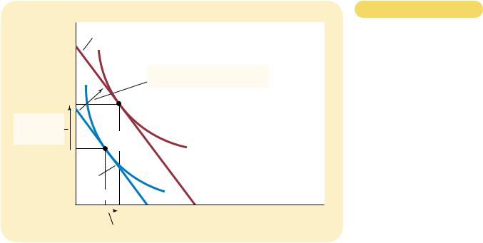
AN INFERIOR GOOD. A good is an inferior good if the consumer buys less of it when his income rises. Here Pepsi is an inferior good: When the consumer’s income increases and the budget constraint shifts outward, the consumer buys more pizza but less Pepsi.
Quantity
of Pepsi
3. . . . but Pepsi consumption falls, making Pepsi an inferior good.
New budget constraint
|
1. When an increase in income shifts the |
Initial |
budget constraint outward . . . |
|
optimum |
|
|
Initial |
|
|
|
budget |
I 1 |
I 2 |
|
constraint |
|
|
|
0 |
|
|
Quantity |
|
|
of Pizza |
2. . . . pizza consumption rises, making pizza a normal good . . . |
|
|
|
|
HOW CHANGES IN PRICES AFFECT
THE CONSUMER’S CHOICES
Let’s now use this model of consumer choice to consider how a change in the price of one of the goods alters the consumer’s choices. Suppose, in particular, that the price of Pepsi falls from $2 to $1 a pint. It is no surprise that the lower price expands the consumer’s set of buying opportunities. In other words, a fall in the price of any good shifts the budget constraint outward.
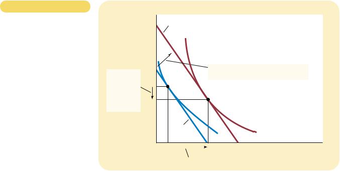
Figure 21-9 considers more specifically how the fall in price affects the budget constraint. If the consumer spends his entire $1,000 income on pizza, then the price of Pepsi is irrelevant. Thus, point A in the figure stays the same. Yet if the consumer spends his entire income of $1,000 on Pepsi, he can now buy 1,000 rather than only 500 pints. Thus, the end point of the budget constraint moves from point B to point D.
Notice that in this case the outward shift in the budget constraint changes its slope. (This differs from what happened previously when prices stayed the same but the consumer’s income changed.) As we have discussed, the slope of the budget constraint reflects the relative price of Pepsi and pizza. Because the price of Pepsi has fallen to $1 from $2, while the price of pizza has remained $10, the consumer can now trade a pizza for 10 rather than 5 pints of Pepsi. As a result, the new budget constraint is more steeply sloped.
How such a change in the budget constraint alters the consumption of both goods depends on the consumer’s preferences. For the indifference curves drawn in this figure, the consumer buys more Pepsi and less pizza.
476 |
PART SEVEN ADVANCED TOPIC |
income and substitution effects work in opposite directions. This conclusion is summarized in Table 21-2.
We can interpret the income and substitution effects using indifference curves.
The income effect is the change in consumption that results from the movement to a higher indifference curve. The substitution effect is the change in consumption that results from being at a point on an indifference curve with a different marginal rate of substitution.
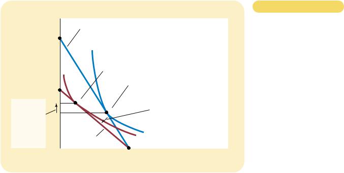
Figure 21-10 shows graphically how to decompose the change in the consumer’s decision into the income effect and the substitution effect. When the price
GOOD |
INCOME EFFECT |
SUBSTITUTION EFFECT |
TOTAL EFFECT |
Pepsi |
Consumer is richer, |
Pepsi is relatively cheaper, so |
|
so he buys more Pepsi. |
consumer buys more Pepsi. |
Income and substitution effects act in same direction, so consumer buys more Pepsi.
Pizza |
Consumer is richer, |
Pizza is relatively more |
|
so he buys more pizza. |
expensive, so consumer |
|
|
buys less pizza. |
Income and substitution effects act in opposite directions, so the total effect on pizza consumption is ambiguous.
Table 21-2 |
|
INCOME AND SUBSTITUTION EFFECTS WHEN THE PRICE OF PEPSI FALLS |
|
|
|
|
|
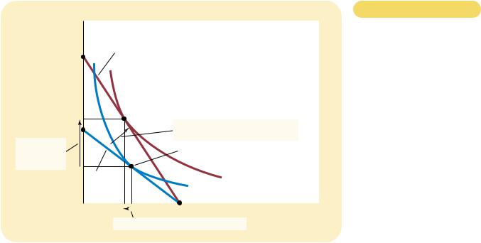
Figur e 21-10
INCOME AND SUBSTITUTION
EFFECTS. The effect of a change in price can be broken down into an income effect and a substitution effect. The substitution effect—the movement along an indifference curve to a point with a different marginal rate of substitution—is shown here as the change from point A to
point B along indifference curve I1. The income effect—the shift to a higher indifference curve—is shown here as the change from point B on
indifference curve I1 to point C on indifference curve I2.
Quantity
of Pepsi
New budget constraint
|
C |
New optimum |
Income |
B |
|
effect |
Initial optimum |
|
|
Substitution |
|
Initial |
|
|
|
|
budget |
|
|
|
effect |
|
|
A |
|
|
constraint |
|
|
|
|
|
|
|
|
|
|
|
|
|
|
|
|
I 2 |
|
|
|
|
|
|
|
|
I 1 |
|
0 |
|
|
|
|
|
|
Quantity |
|
|
Substitution effect |
of Pizza |
|
|
|
|
|
|
|
|
|
Income effect
CHAPTER 21 THE THEORY OF CONSUMER CHOICE |
477 |
of Pepsi falls, the consumer moves from the initial optimum, point A, to the new optimum, point C. We can view this change as occurring in two steps. First, the consumer moves along the initial indifference curve I1 from point A to point B. The consumer is equally happy at these two points, but at point B, the marginal rate of substitution reflects the new relative price. (The dashed line through point B reflects the new relative price by being parallel to the new budget constraint.) Next, the consumer shifts to the higher indifference curve I2 by moving from point B to point C. Even though point B and point C are on different indifference curves, they have the same marginal rate of substitution. That is, the slope of the indifference curve I1 at point B equals the slope of the indifference curve I2 at point C.
Although the consumer never actually chooses point B, this hypothetical point is useful to clarify the two effects that determine the consumer’s decision. Notice that the change from point A to point B represents a pure change in the marginal rate of substitution without any change in the consumer’s welfare. Similarly, the change from point B to point C represents a pure change in welfare without any change in the marginal rate of substitution. Thus, the movement from A to B shows the substitution effect, and the movement from B to C shows the income effect.
DERIVING THE DEMAND CURVE
We have just seen how changes in the price of a good alter the consumer’s budget constraint and, therefore, the quantities of the two goods that he chooses to buy. The demand curve for any good reflects these consumption decisions. Recall that a demand curve shows the quantity demanded of a good for any given price. We can view a consumer’s demand curve as a summary of the optimal decisions that arise from his budget constraint and indifference curves.
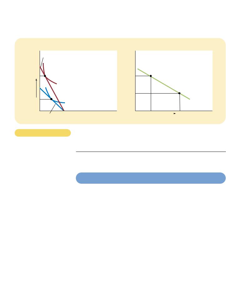
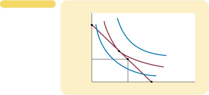
For example, Figure 21-11 considers the demand for Pepsi. Panel (a) shows that when the price of a pint falls from $2 to $1, the consumer’s budget constraint shifts outward. Because of both income and substitution effects, the consumer increases his purchases of Pepsi from 50 to 150 pints. Panel (b) shows the demand curve that results from this consumer’s decisions. In this way, the theory of consumer choice provides the theoretical foundation for the consumer’s demand curve, which we first introduced in Chapter 4.
Although it is comforting to know that the demand curve arises naturally from the theory of consumer choice, this exercise by itself does not justify developing the theory. There is no need for a rigorous, analytic framework just to establish that people respond to changes in prices. The theory of consumer choice is, however, very useful. As we see in the next section, we can use the theory to delve more deeply into the determinants of household behavior.
QUICK QUIZ: Draw a budget constraint and indifference curves for Pepsi and pizza. Show what happens to the budget constraint and the consumer’s optimum when the price of pizza rises. In your diagram, decompose the change into an income effect and a substitution effect.
478 |
PART SEVEN ADVANCED TOPIC |
|
|
|
(a) The Consumer’s Optimum |
(b) The Demand Curve for Pepsi |
|
Quantity |
|
Price of |
|
of Pepsi |
New budget constraint |
Pepsi |
|
|
|
I 1
0Initial budget constraint
Figur e 21-11
Quantity |
0 |
50 |
|
150 |
Quantity |
|
of Pizza |
|
|
|
|
of Pepsi |
DERIVING THE DEMAND CURVE. Panel (a) shows that when the price of Pepsi falls from $2 to $1, the consumer’s optimum moves from point A to point B, and the quantity of Pepsi consumed rises from 50 to 150 pints. The demand curve in panel (b) reflects this relationship between the price and the quantity demanded.
FOUR APPLICATIONS
Now that we have developed the basic theory of consumer choice, let’s use it to shed light on four questions about how the economy works. These four questions might at first seem unrelated. But because each question involves household decisionmaking, we can address it with the model of consumer behavior we have just developed.
DO ALL DEMAND CURVES SLOPE DOWNWARD?
Normally, when the price of a good rises, people buy less of it. Chapter 4 called this usual behavior the law of demand. This law is reflected in the downward slope of the demand curve.
As a matter of economic theory, however, demand curves can sometimes slope upward. In other words, consumers can sometimes violate the law of demand and buy more of a good when the price rises. To see how this can happen, consider Figure 21-12. In this example, the consumer buys two goods—meat and potatoes. Initially, the consumer’s budget constraint is the line from point A to point B. The optimum is point C. When the price of potatoes rises, the budget constraint shifts inward and is now the line from point A to point D. The optimum is now point E.
480 |
PART SEVEN ADVANCED TOPIC |
Figur e 21-13
THE WORK-LEISURE DECISION.
This figure shows Sally’s budget constraint for deciding how much to work, her indifference curves for consumption and leisure, and her optimum.
Consumption
$5,000
Optimum
I 3
2,000
I 2
I 1
0 |
60 |
100 |
Hours of Leisure |
HOW DO WAGES AFFECT LABOR SUPPLY?
So far we have used the theory of consumer choice to analyze how a person decides how to allocate his income between two goods. We can use the same theory to analyze how a person decides to allocate his time between work and leisure.
Consider the decision facing Sally, a freelance software designer. Sally is awake for 100 hours per week. She spends some of this time enjoying leisure—rid- ing her bike, watching television, studying economics, and so on. She spends the rest of this time at her computer developing software. For every hour she spends developing software, she earns $50, which she spends on consumption goods. Thus, her wage ($50) reflects the tradeoff Sally faces between leisure and consumption. For every hour of leisure she gives up, she works one more hour and gets $50 of consumption.
Figure 21-13 shows Sally’s budget constraint. If she spends all 100 hours enjoying leisure, she has no consumption. If she spends all 100 hours working, she earns a weekly consumption of $5,000 but has no time for leisure. If she works a normal 40-hour week, she enjoys 60 hours of leisure and has weekly consumption of $2,000.
Figure 21-13 uses indifference curves to represent Sally’s preferences for consumption and leisure. Here consumption and leisure are the two “goods” between which Sally is choosing. Because Sally always prefers more leisure and more consumption, she prefers points on higher indifference curves to points on lower ones. At a wage of $50 per hour, Sally chooses a combination of consumption and leisure represented by the point labeled “optimum.” This is the point on the budget constraint that is on the highest possible indifference curve, which is curve I2.
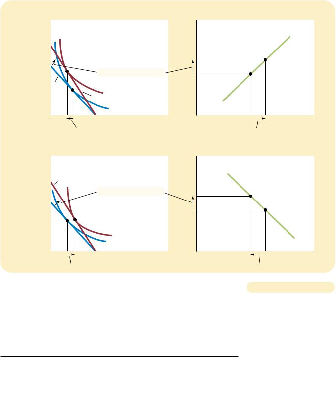
Now consider what happens when Sally’s wage increases from $50 to $60 per hour. Figure 21-14 shows two possible outcomes. In each case, the budget constraint, shown in the left-hand graph, shifts outward from BC1 to BC2. In the process, the budget constraint becomes steeper, reflecting the change in relative
CHAPTER 21 |
THE THEORY OF CONSUMER CHOICE |
481 |
(a) For a person with these preferences . . . |
. . . the labor supply curve slopes upward. |
|
Consumption |
Wage |
|
Labor |
|
supply |
|
1. When the wage rises . . . |
|
BC1 |
|
I 2 |
|
BC2 |
|
I 1 |
0 |
|
|
Hours of |
0 |
|
|
|
|
Hours of Labor |
|
2 |
hours of leisure decrease |
Leisure |
|
3 |
and hours of labor increase. |
Supplied |
|
|
|
|
|
(b) For a person with these preferences . . . |
|
|
. . . the labor supply curve slopes backward. |
Consumption |
Wage |
BC2 |
|
|
1. When the wage rises . . . |
BC1 |
Labor |
supply |
|
I 2 |
|
I 1 |
0 |
|
|
Hours of |
0 |
|
|
|
Hours of Labor |
|
2. . . . hours of leisure increase . . . |
Leisure |
|
3. . . . and hours of labor decrease. |
Supplied |
|
|
|
|
AN INCREASE IN THE WAGE. |
The two panels of this figure show how a person might |
|
|
|
|
|
|
Figur e 21-14 |
respond to an increase in the wage. The graphs on the left show the consumer’s initial |
|
|
|
|
|
|
budget constraint BC1 and new budget constraint BC2, as well as the consumer’s optimal choices over consumption and leisure. The graphs on the right show the resulting labor supply curve. Because hours worked equal total hours available minus hours of leisure, any change in leisure implies an opposite change in the quantity of labor supplied. In panel (a), when the wage rises, consumption rises and leisure falls, resulting in a labor supply curve that slopes upward. In panel (b), when the wage rises, both consumption and leisure rise, resulting in a labor supply curve that slopes backward.
price: At the higher wage, Sally gets more consumption for every hour of leisure that she gives up.
Sally’s preferences, as represented by her indifference curves, determine the resulting responses of consumption and leisure to the higher wage. In both panels,