464 |
PART SEVEN ADVANCED TOPIC |
a more complete understanding of demand, just as the theory of the competitive firm in Chapter 14 provides a more complete understanding of supply.
One of the Ten Principles of Economics discussed in Chapter 1 is that people face tradeoffs. The theory of consumer choice examines the tradeoffs that people face in their role as consumers. When a consumer buys more of one good, he can afford less of other goods. When he spends more time enjoying leisure and less time working, he has lower income and can afford less consumption. When he spends more of his income in the present and saves less of it, he must accept a lower level of consumption in the future. The theory of consumer choice examines how consumers facing these tradeoffs make decisions and how they respond to changes in their environment.
After developing the basic theory of consumer choice, we apply it to several questions about household decisions. In particular, we ask:
Do all demand curves slope downward?
How do wages affect labor supply?
How do interest rates affect household saving?
Do the poor prefer to receive cash or in-kind transfers?
At first, these questions might seem unrelated. But, as we will see, we can use the theory of consumer choice to address each of them.
THE BUDGET CONSTRAINT :
WHAT THE CONSUMER CAN AFFORD
Most people would like to increase the quantity or quality of the goods they con- sume—to take longer vacations, drive fancier cars, or eat at better restaurants. People consume less than they desire because their spending is constrained, or limited, by their income. We begin our study of consumer choice by examining this link between income and spending.
To keep things simple, we examine the decision facing a consumer who buys only two goods: Pepsi and pizza. Of course, real people buy thousands of different kinds of goods. Yet assuming there are only two goods greatly simplifies the problem without altering the basic insights about consumer choice.
We first consider how the consumer’s income constrains the amount he spends on Pepsi and pizza. Suppose that the consumer has an income of $1,000 per month and that he spends his entire income each month on Pepsi and pizza. The price of a pint of Pepsi is $2, and the price of a pizza is $10.
Table 21-1 shows some of the many combinations of Pepsi and pizza that the consumer can buy. The first line in the table shows that if the consumer spends all his income on pizza, he can eat 100 pizzas during the month, but he would not be able to buy any Pepsi at all. The second line shows another possible consumption bundle: 90 pizzas and 50 pints of Pepsi. And so on. Each consumption bundle in the table costs exactly $1,000.
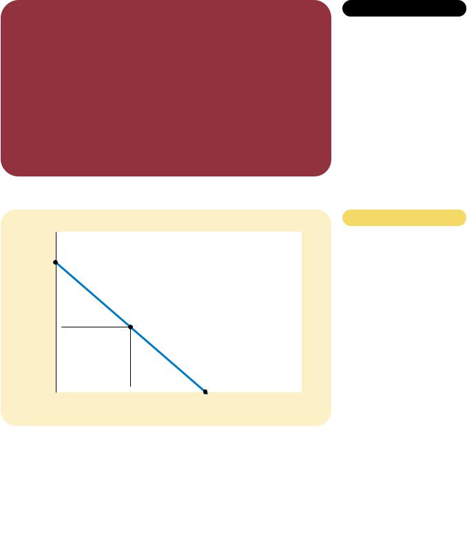
Figure 21-1 graphs the consumption bundles that the consumer can choose. The vertical axis measures the number of pints of Pepsi, and the horizontal axis
466 |
PART SEVEN ADVANCED TOPIC |
The slope of the budget constraint measures the rate at which the consumer can trade one good for the other. Recall from the appendix to Chapter 2 that the slope between two points is calculated as the change in the vertical distance divided by the change in the horizontal distance (“rise over run”). From point A to point B, the vertical distance is 500 pints, and the horizontal distance is 100 pizzas. Thus, the slope is 5 pints per pizza. (Actually, because the budget constraint slopes downward, the slope is a negative number. But for our purposes we can ignore the minus sign.)
Notice that the slope of the budget constraint equals the relative price of the two goods—the price of one good compared to the price of the other. A pizza costs 5 times as much as a pint of Pepsi, so the opportunity cost of a pizza is 5 pints of Pepsi. The budget constraint’s slope of 5 reflects the tradeoff the market is offering the consumer: 1 pizza for 5 pints of Pepsi.
QUICK QUIZ: Draw the budget constraint for a person with income of $1,000 if the price of Pepsi is $5 and the price of pizza is $10. What is the slope of this budget constraint?
PREFERENCES: WHAT THE CONSUMER WANTS
indif fer ence cur ve
a curve that shows consumption bundles that give the consumer the same level of satisfaction
Our goal in this chapter is to see how consumers make choices. The budget constraint is one piece of the analysis: It shows what combination of goods the consumer can afford given his income and the prices of the goods. The consumer’s choices, however, depend not only on his budget constraint but also on his preferences regarding the two goods. Therefore, the consumer’s preferences are the next piece of our analysis.
REPRESENTING PREFERENCES WITH
INDIFFERENCE CURVES
The consumer’s preferences allow him to choose among different bundles of Pepsi and pizza. If you offer the consumer two different bundles, he chooses the bundle that best suits his tastes. If the two bundles suit his tastes equally well, we say that the consumer is indifferent between the two bundles.
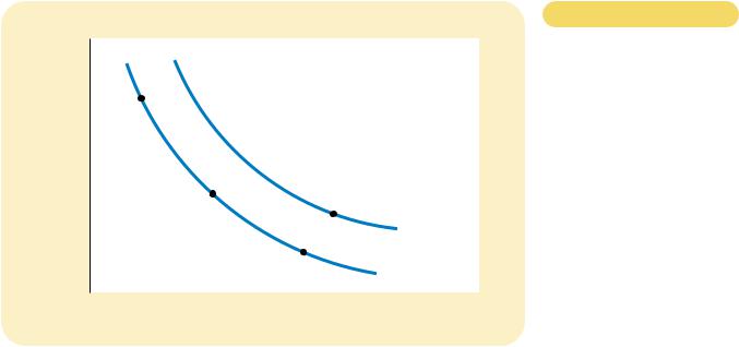
Just as we have represented the consumer’s budget constraint graphically, we can also represent his preferences graphically. We do this with indifference curves. An indifference curve shows the bundles of consumption that make the consumer equally happy. In this case, the indifference curves show the combinations of Pepsi and pizza with which the consumer is equally satisfied.
Figure 21-2 shows two of the consumer’s many indifference curves. The consumer is indifferent among combinations A, B, and C, because they are all on the same curve. Not surprisingly, if the consumer’s consumption of pizza is reduced, say from point A to point B, consumption of Pepsi must increase to keep him equally happy. If consumption of pizza is reduced again, from point B to point C, the amount of Pepsi consumed must increase yet again.
468 |
PART SEVEN ADVANCED TOPIC |
FOUR PROPERTIES OF INDIFFERENCE CURVES
Because indifference curves represent a consumer’s preferences, they have certain properties that reflect those preferences. Here we consider four properties that describe most indifference curves:
Property 1: Higher indifference curves are preferred to lower ones. Consumers usually prefer more of something to less of it. (That is why we call this something a “good” rather than a “bad.”) This preference for greater quantities is reflected in the indifference curves. As Figure 21-2 shows, higher indifference curves represent larger quantities of goods than lower indifference curves. Thus, the consumer prefers being on higher indifference curves.
Property 2: Indifference curves are downward sloping. The slope of an indifference curve reflects the rate at which the consumer is willing to substitute one good for the other. In most cases, the consumer likes both goods. Therefore, if the quantity of one good is reduced, the quantity of the other good must increase in order for the consumer to be equally happy. For this reason, most indifference curves slope downward.
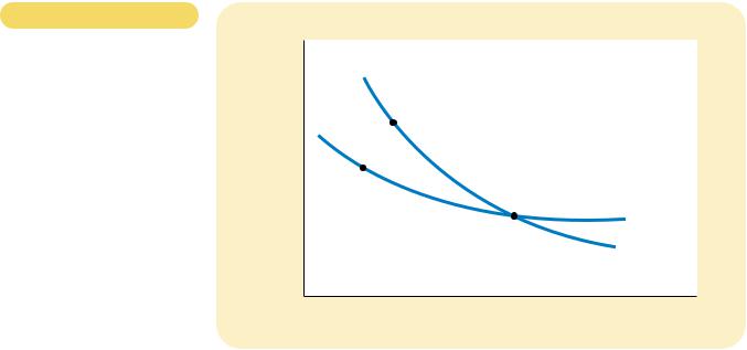
Property 3: Indifference curves do not cross. To see why this is true, suppose that two indifference curves did cross, as in Figure 21-3. Then, because point A is on the same indifference curve as point B, the two points would make the consumer equally happy. In addition, because point B is on the same indifference curve as point C, these two points would make the consumer equally happy. But these conclusions imply that points A and C would also make the consumer equally happy, even though point C has more of both goods. This contradicts our assumption that the consumer always prefers more of both goods to less. Thus, indifference curves cannot cross.
Figur e 21-3
THE IMPOSSIBILITY OF
INTERSECTING INDIFFERENCE
CURVES. A situation like this can never happen. According to these indifference curves, the consumer would be equally satisfied at points A, B, and C, even though point C has more of both goods than point A.
CHAPTER 21 THE THEORY OF CONSUMER CHOICE |
469 |
MRS = 1 |
|
B |
|
1 |
Indifference |
|
|
|
|
curve |
0 |
2 |
3 |
6 |
7 |
Quantity |
|
|
|
|
|
of Pizza |
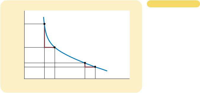
Property 4: Indifference curves are bowed inward. The slope of an indifference curve is the marginal rate of substitution—the rate at which the consumer is willing to trade off one good for the other. The marginal rate of substitution (MRS) usually depends on the amount of each good the consumer is currently consuming. In particular, because people are more willing to trade away goods that they have in abundance and less willing to trade away goods of which they have little, the indifference curves are bowed inward. As an example, consider Figure 21-4. At point A, because the consumer has a lot of Pepsi and only a little pizza, he is very hungry but not very thirsty. To induce the consumer to give up 1 pizza, the consumer has to be given 6 pints of Pepsi: The marginal rate of substitution is 6 pints per pizza. By contrast, at point B, the consumer has little Pepsi and a lot of pizza, so he is very thirsty but not very hungry. At this point, he would be willing to give up 1 pizza to get 1 pint of Pepsi: The marginal rate of substitution is 1 pint per pizza. Thus, the bowed shape of the indifference curve reflects the consumer’s greater willingness to give up a good that he already has in large quantity.
Figur e 21-4
BOWED INDIFFERENCE CURVES.
Indifference curves are usually bowed inward. This shape implies that the marginal rate of substitution (MRS) depends on the quantity of the two goods the consumer is consuming. At point A, the consumer has little pizza and much Pepsi, so he requires a lot of extra Pepsi to induce him to give up one of the pizzas: The marginal rate of substitution is
6 pints of Pepsi per pizza. At point B, the consumer has much pizza and little Pepsi, so he requires only a little extra Pepsi to induce him to give up one of the pizzas: The marginal rate of substitution is 1 pint of Pepsi per pizza.
TWO EXTREME EXAMPLES OF INDIFFERENCE CURVES
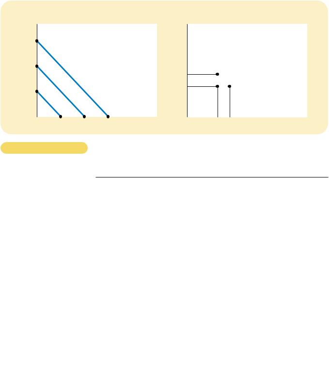
The shape of an indifference curve tells us about the consumer’s willingness to trade one good for the other. When the goods are easy to substitute for each other, the indifference curves are less bowed; when the goods are hard to substitute, the indifference curves are very bowed. To see why this is true, let’s consider the extreme cases.
Per fect Substitutes Suppose that someone offered you bundles of nickels and dimes. How would you rank the different bundles?

|
|
|
CHAPTER 21 THE THEORY OF CONSUMER CHOICE |
471 |
|
|
|
|
|
|
|
|
F Y I |
|
|
|
|
|
|
Utility: An |
|
We have used indifference |
curves, bundles of goods on higher indifference curves pro- |
|
|
Alternative |
|
curves to represent the con- |
vide higher utility. Because the consumer is equally happy |
|
|
Way to |
|
sumer’s preferences. Another |
with all points on the same indifference curve, all these |
|
|
Represent a |
|
common way to represent pref- |
bundles provide the same utility. Indeed, you can think of an |
|
|
Consumer’s |
|
erences is with the concept of |
indifference curve as an “equal-utility” curve. The slope of |
|
|
Preferences |
|
|
|
|
utility. Utility is an abstract mea- |
the indifference curve (the marginal rate of substitution) re- |
|
|
|
|
|
|
|
|
sure of the satisfaction or happi- |
flects the marginal utility generated by one good compared |
|
|
|
|
ness that a consumer receives |
to the marginal utility generated by the other good. |
|
|
|
|
|
from a bundle of goods. Econo- |
When economists discuss the theory of consumer |
|
|
|
|
mists say that a consumer |
choice, they might express the theory using different words. |
|
|
|
|
prefers one bundle of goods to |
One economist might say that the goal of the consumer is to |
|
|
|
|
another if the first provides |
maximize utility. Another might say that the goal of the con- |
|
|
|
|
more utility than the second. |
sumer is to end up on the highest possible indifference |
|
|
Indifference curves and utility are closely related. Be- |
curve. In essence, these are two ways of saying the same |
|
|
cause the consumer prefers points on higher indifference |
thing. |
|
|
|
|
|
|
|
|
|
typically, the indifference curves are bowed inward, but not so bowed as to become right angles.
QUICK QUIZ: Draw some indifference curves for Pepsi and pizza. Explain the four properties of these indifference curves.
OPTIMIZATION: WHAT THE CONSUMER CHOOSES
The goal of this chapter is to understand how a consumer makes choices. We have the two pieces necessary for this analysis: the consumer’s budget constraint and the consumer’s preferences. Now we put these two pieces together and consider the consumer’s decision about what to buy.
THE CONSUMER’S OPTIMAL CHOICES
Consider once again our Pepsi and pizza example. The consumer would like to end up with the best possible combination of Pepsi and pizza—that is, the combination on the highest possible indifference curve. But the consumer must also end up on or below his budget constraint, which measures the total resources available to him.
Figure 21-6 shows the consumer’s budget constraint and three of his many indifference curves. The highest indifference curve that the consumer can reach (I2 in the figure) is the one that just barely touches the budget constraint. The point at which this indifference curve and the budget constraint touch is called the optimum. The consumer would prefer point A, but he cannot afford that point because