Словари и журналы / Психологические журналы / p33Journal of Occupational and Organizational Psychology

34 Christian Dormann and Dieter Zapf

Figure 1. The development of psychological complaints (adopted from Mohr, 1991)

1998). Although no rigorous propositions were made regarding the particular stressors that may trigger the chain of stress reactions, the ordering of stress reactions was clearly described. Leiter and Maslach (1988) proposed that stressors first lead to emotional exhaustion, which then leads to depersonalization which, in turn, causes a reduced sense of personal accomplishment. In contrast, Golembiewski, Munzenrider, and Stevenson (1986) suggested that the sequence starts with depersonalization, followed by reduced personal accomplishment, and finally emotional exhaustion. In testing these models, Lee and Ashforth (1993) presented one of the few longitudinal studies which analysed such mediation mechanisms, and the results were in favour of the Leiter and Maslach model. Dignam and West (1988) presented another two-wave study, which analysed mediation among stress reaction. They investigated whether stressors first lead to burnout. In this study, burnout was a latent factor with emotional exhaustion and depersonalization as indicators. They hypothesized that when burnout symptoms occur, they cause poor health. Support for this hypothesis was only found in cross-sectional analyses, but not when longitudinal models were applied.

A theoretical model that has not yet been subjected to empirical investigation was developed by Mohr (1986, 1991). In parts, this model is tested in the present study. Therefore, it is now described in more detail.

Mohr’s (1986, 1991) model suggests that stressors at work are the starting points of a temporarily ordered sequence of different stress reactions which are causally connected. First, irritation emerges, which then leads to a decrease in self-esteem and an increase in anxiety. Anxiety leads to depressive symptoms and further reduces self-esteem, which also leads to an increase in depressive symptoms. Psychosomatic complaints are also part of the model suggested by Mohr, which is shown in Fig. 1. The

crucial point in this model is that increases in different responses to stressors at work occur not only with varying delays, but that an increase in irritation causes an increase in anxiety and a decrease in self-esteem, which then subsequently cause an increase in depressive symptoms.

Mohr (1991) cited prior evidence suggesting that social isolation might be critical in the development of depressive symptoms. She further supposed that social conflicts are relevant in the development of irritation. This is in line with the proposition of others (e.g. Kuhl & Helle, 1994), who also mentioned social isolation as a precursor of depressive symptoms. Schonfeld (1992) found that confrontations initiated by insolent students were a precursor of depression in a sample of first-year female teachers. For professional-managerial women, Snapp (1992) reported that trouble with the boss or subordinates was positively related to depression. Social conflicts at work were also related to depression in studies by Heinisch and Jex (1997) and Karasek and Theorell (1990). Social isolation and social conflicts are examples of social stressors (Frese & Zapf, 1987). Social stressors may thus play a critical role in the development of irritation and subsequent depressive symptoms.

Compared to other work stressors such as time pressure, role conflict or role ambiguity, there is little research on social stressors in organizations. Social stressors consist of social animosities, conflicts with co-workers and supervisors, unfair behaviour, and a negative group climate. There is reason to believe that social stressors may have strong effects on strains. Zapf and Frese (1991) have shown that social stressors are relatively strong predictors of depressive symptoms in comparison to various task stressors. In a diary study by Schwartz and Stone (1993), 75%of all recorded work-related events that indiviudals assessed as harmful were related to negative social interactions with colleagues, supervisors, and clients. Social or interpersonal stressors were an important predictor of other psychological strain variables in the studies of Heinisch and Jex (1997), Keashly, Hunter, and Harvey (1997), Spector (1987), Spector and Jex (1998), and Zapf, Seifert, Schmutte, Mertini, and Holz(2001). Moreover, research on social support at work repeatedly demonstrated that lack of support has negative consequences, underscoring the importance of personal relationships in organizations in comparison with task-related and organization-related issues (e.g. Abdel-Halim, 1982; Ganster, Fusilier, &Mayes, 1986; LaRocco, House, & French, 1980). Social stressors and lack of support are not identical. Although social stressors and social support tend to be negatively correlated (e.g. Dormann &Zapf, 1999), there are exceptions to the rule. For example, a supervisor who pushes all the time could nevertheless be very supportive in getting the job done.

One can assume that there is a relationship between job stressors and social stressors. If there is time pressure, there may be a supervisor being responsible for it. In particular, one may associate role conflict and role ambiguity with the social system at work. However, most researchers consider them to be related to the task structure and the organization of work focusing on unclear or contradictory task goals. Therefore, these concepts are clearly distinct from social stressors comprising social conflicts, personal animosities or unfair behaviour.

The model of Mohr (1986, 1991) is quite complex and a huge sample size would be necessary to test the whole model in a longitudinal fashion. Therefore, only the relationships among social stressors, irritation, and depressive symptoms were investigated in the present study. This corresponds to the grey-shaded area in Fig. 1. Although the model does not include a direct effect of irritation on depressive symptoms, such an effect would be established if the two mediating variables anxiety and self-esteem were excluded from the model. This represents hypothesis 1 of the present study.

36 Christian Dormann and Dieter Zapf

Figure 2. The baseline model (error-autocorrelations of observed indicators omitted for clarity)

Hypothesis 1: Social stressors at work affect irritation, and irritation affects depressive symptoms.

Moreover, it is assumed that there is a pure mediation mechanism. That is, as long as irritation is included in a model, a direct effect of social stressors on depressive symptoms should be absent. This represents hypothesis 2 of the present study.

Hypothesis 2: Social stressors do not directly affect depressive symptoms.

In organizational stress research, authors have repeatedly commented on the methodological shortcomings of many studies (e.g. Frese & Zapf, 1988; Kasl, 1978; Spector, 1992). Among other things, authors have suggested (a) using longitudinal designs to analyse causal effects; (b) taking into account that there may be third variables responsible for the stressor–strain relationship; (c) taking reverse causation into account, that is, the possibility that some strains may affect the stressors perceived at one’s job; and (d) considering the time lag necessary for a stressor to develop its effect on strain.

These issues are all considered in the present paper. The first two hypotheses were tested using a multi-wave design, which was based on a representative sample of the working population of Dresden in Germany.

Hypotheses 1 and 2 are shown in Fig. 2. In this figure, social stressors, irritation and depressive symptoms are measured at three time points and it is assumed that the variables have some stability, reflected by the arrows from social stressors Time 1 to social stressors Time 2, from social stressors Time 2 to social stressors Time 3, etc. According to hypothesis 1 there are causal paths (arrows) from social stressors to irritation and from irritation to depressive symptoms. According to hypothesis 2, there are no direct causal paths from social stressors to depressive symptoms.

One shortcoming of many published longitudinal studies is that the potential of longitudinal data to rule out alternative explanations for the hypotheses under study

has often not been used (exceptions are, e.g., Dignam & West, 1988; Marcelissen, Winnubst, Buunk, & de Wolff, 1988). The most important alternative explanations refer to reversed causation and third variables. The latter means that an observed relationship is due to the effect a third variable has on the independent and the dependent variable. An example is negative affectivity which has recently been hypothesized to explain self-reported stressor–strain relations (e.g. Burke, Brief, & George, 1993). If third variables, which are held responsible for the spuriousness of a relation, are known and have been measured, the treatment of these variables is straightforward. They can, for example, be partialled out in correlative designs (see, however, Spector, Zapf, Chen, & Frese, 2000). The problem is that researchers do not always have all the relevant information about a causal system, so it can always be argued that a relevant third variable has been left out from the analysis. Therefore, one cannot be sure whether or not a causal interpretation of empirically derived relationships is valid.

There are, however, some methods available when considering the effects of third variables that have not actually been measured (e.g. Dormann, 2001; Dwyer, 1983; Finkel, 1995; Kenny, 1975, 1979). They provide means of protecting one’s findings from special kinds of omitted third variable explanations. Basically, such methods rest on assumptions regarding the properties of the unmeasured third variable that should be ruled out as a source of spuriousness. Dormann showed how an extended version of the synchronous common factor (SCF) model, which is the basic model underlying the cross-lagged panel correlation technique (Kenny, 1975), can be used to rule out unmeasured variables as sources of spuriousness when more than two variables, each of which is measured at least twice, are analysed. Compared to the SCF, the model proposed byDormann is less restrictive and therefore called the ‘less restrictive synchronous common factor’ (LRSCF) model. The LRSCFmodel is described in some more detail in the Methods section, but it should be noted here that an LRSCF represents a latent variable, (a) which affects the variables of interest (i.e. social stressors, irritation, and depressive symptoms in this instance), (b) which maychange over time to some degree, and (c) which is not actually measured but is estimated on the basis of its relations with other variables. According to Dormann, the so-called occasion factors, which are shown in Fig. 3, can be considered as a special case of LRSCF.

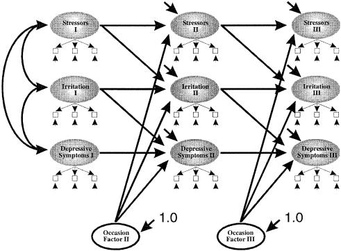
Occasion factors represent third variables that affect other variables in a given situation and which are completely unstable (Dwyer, 1983). The impact of good weather may be an example. Good weather may reduce the level of depressive symptoms, may make individuals feel less irritated, and may even reduce the number of social conflicts because everybody is in a good mood. In Fig. 3, this is shown by causal paths from the occasion factors on social stressors, irritation and depressive symptoms. If weather is assumed to be a completely unstable variable this means that current weather does not allow a prediction about what the weather will be like in the future. In Fig. 3, this is shown by the fact that the occasion factor Time 2 is unrelated to the occasion factor Time 3.

A more general LRSCF model is shown in Fig. 4. In addition to the occasion factor model, this model assumes that the third variable possesses some stability over time shown by the causal path from LRSCF II to LRSCF III. Assume, for example, that time pressure is responsible for the relationships proposed in hypothesis 1. Time pressure causes a deterioration in the social climate and thus increases social stressors. In addition, it causes irritation and depressive symptoms. If time pressure is not included in the model, its effects may mistakenly appear as causal effects between social

38 Christian Dormann and Dieter Zapf

Figure 3. Occasion factor model (error-autocorrelations of observed indicators omitted for clarity)

stressors and irritation and between irritation and depressive symptoms as proposed in hypothesis 1, although there is, in reality, no causal relationship at all among these variables. The LRSCFs in Fig. 4 stand for any variable which has similar effects as in the example given. Dormann (2001) has shown that the model presented in Fig. 4 is identified and can be analysed using structural equation modelling.

In the present study, occasion factor models and LRSCF models as proposed by Dormann (2001) were investigated leading to hypothesis 3.

Hypothesis 3: Hypothesis 1 is valid even if occasion factors and LRSCfactors are taken into account.

In the stress literature, various third variables have been suggested to explain stressor– strain relations (e.g. Brief, Burke, George, Robinson, & Webster, 1988; Kasl, 1986; Spector, 1992; Zapf, 1989). Examples are social status, social desirability, negative affectivity or mood. The unmeasured third variables of the present study may stand for one or more of these variables.

Another shortcoming of previous longitudinal studies is the issue of reversed causation, which is often not tested. Several explanations regarding reversed causation can be brought forward. Mohr (1991) argued that stressors and irritation might be reciprocally related. For instance, irritated employees may lack resources to cope with social conflicts. They may focus on the personal relation rather than on the tasks they have to deal with, which may then lead to conflict escalation (Glasl, 1994).

Figure 4. LRSCF model (error-autocorrelations of observed indicators omitted for clarity)

Sacco, Dumont, and Dow (1993) showed that people respond negatively to depressed individuals. Accordingly, the more depressed employees are, the more supervisors or colleagues might behave in a socially stressful way. In addition, in his review and reformulation of the frustration–aggression model, Berkowitz (1989, p. 71) suggests, ‘[. . .] somewhat tentatively, that any kind of negative affect, sadness as well as depression and agitated irritability, will produce aggressive inclinations [. . .].’ Aggressive behaviour may poison the social atmosphere at work and thereby increase subsequent social stressors, implying that depressive symptoms and irritation may have reversed effects on social stressors. Longitudinal studies are the only means to test for reversed causation in field research. Reversed causation is considered in hypothesis 4.

Hypothesis 4: Hypothesis 1 is valid, even if possible reversed causation mechanisms are taken into account.

Finally, nothing is really known about adequate time lags because, among the studies reviewed by Zapf, Dormann, and Frese (1996), this was only tested in the studies by Schonfeld (1992) and Kohn and Schooler (1982), who tested synchronous and lagged effects. Often, time lags in longitudinal studies are pragmatically selected. Most often, 1-year lags were used (e.g. Zapf et al., 1996). The present study was based on a multi-wave design, which allows one to systematically test the most adequate time lag for social stressors to affect irritation and for irritation to affect depressive symptoms. The lack of systematic attempts to investigate adequate time lags did not allow us to develop firm hypotheses, so this issue was investigated in an explorative manner.

40 Christian Dormann and Dieter Zapf

Methods

The data of the present study were taken from the AHUS project (a German acronym for ‘active behaviour in a radical change situation’), which started in 1990.1 At this time, the unification of East and West Germany was close at hand. The primary aim of the AHUS project was to analyse how citizens of former East Germany would cope with the change processes triggered by the unification. In particular, it was expected that a great variety of changes was likely to occur concerning working conditions because the capitalistic economic system of former West Germany had to be carried over into socialist East Germany.

The study now consists of six waves of data collection. The first wave took place in July/ August 1990. At this time, West German currency was introduced into East Germany. Four months later, in October/November 1990, the second wave of data collection was carried out. At this time, the unification of East and West Germany had just occurred a few weeks earlier. The third wave was collected 8 months later, in July/August 1991. From then on, separated by lags of 1 year each; wave 4 took place in July/August 1992 and wave 5 in July/August 1993. The last wave of data collection was carried out in July/August 1995. Due to the sampling procedure described next, however, all analyses are restricted to waves 3–6, which are labelled Time 1 to Time 4 for ease of presentation.

Sample

Data were collected in Dresden, one of the three largest cities in the former East Germany. To achieve representativeness, a random route sampling method was applied. In randomly selected streets, collaborators of the project visited every fourth apartment (in smaller houses every third). When residents were not at home, at least two additional calls were made. Everyone who was employed full-time and was between the ages of 18 and 65 was invited to participate. Thus, in several instances more than one person from each household was included in the study. This was the case in about one-third of the households contacted, leading to about 48.6%cases where a partner was part of the sample. Anonymity was ensured by creating a personal code, which was necessary to correctly assign data from subsequent waves. People were paid for participation: 30DM at the first wave of data collection and 50DM (approximately 25 euros) at each subsequent one. About 33%refused participation.

In wave 1, the sample consisted of 365 residents of Dresden. In wave 2, 202 additional subjects were sampled using the same procedure as in wave 1. In 1990, there were 307 935 residents of Dresden in work (Statistical Office of the Federal State of Saxonia, personal communication, 21 March 2000). Given the full sample of 567 participants, this corresponds to a participation rate of 0.184%. The sample is representative of the working population of Dresden with respect to age, social class, and male/female percentage at work (Frese et al., 1996). There were 52.4%male and 47.6%female participants. Age ranged from 16 to 63 years (M=39.50, SD=11.54; in 1990). Most participants worked in public or private services (35.9%), followed by a group employed in trade or manufacturing enterprises (30.9%). Overall, there were 18.9% office workers in jobs that required few qualifications, 27.4% managers or professionals with high qualifications, 12.5%higher level public servants, mostly employed in schools and universities, and 16.5%skilled and 14.9%unskilled blue collar workers.

Measures

At each measurement point, subjects were asked to fill out a questionnaire, which consisted of several different parts. From the extensive set of variables available, three scales were taken to investigate the models proposed so far. These three measures are described next.

1The on-going project AHUS (Aktives Handeln in einer Umbruchsituation—active behaviour in a radical change situation) is supported by the Deutsche Forschungsgemeinschaft (DFG, No. Fr 638/6-6) (principal investigator: Michael Frese). One prior publication (Dormann & Zapf, 1999) partly overlaps with the present article in as much as the last wave analysed by Dormann and Zapf (1999), who analysed the interaction of social stressors and social support, represents the Ž rst wave analysed in the present article. Other publications and proposed publications on the basis of the AHUS project do not overlap with the present study. They were either concerned with personal initiative (e.g. Frese, Fay, Hilburger, Leng, & Tag, 1997; M. Frese, H. Garst, & D. Fay, unpublished; Frese, Kring, Soose, & Zempel, 1996) or with growth models of stressors and strains (Garst, Frese, & Molenaar, 2000).

Social stressors

Items of social stressors were developed by Frese and Zapf (1987). Three items were used to limit the complexity of LISREL models and to retain an acceptable ratio of subjects per estimated parameter (‘I have to work together with people who do not understand fun’, ‘My supervisor always assigns the pleasant tasks to particular people’, and ‘One has to pay for the mistakes of others’). The questions required a response on a 5-point scale that ranged from 1 =‘not at all true’ to 5 =‘absolutely true’. Cronbach’s a values for the 3-item scale ranged from a minimum of .64 obtained at Time 1 to a maximum of .70 obtained at Time 4. The correlation of a scale based on the three items selected in our study with the original 8-item scale (a=.80) was r=.86 (N=584) in another study (C. Dormann & D. Zapf, unpublished).

Previous research has shown that the social stressor scale is not affected by verbal fluency, social desirability and political attitudes. The validity of this scale has also been established with regard to job characteristics, social support and health variables (Dormann, Zapf, & Isic, in press; Frese & Zapf, 1987; Zapf & Frese, 1991; Zapf et al., 2001). In addition, the study by Frese and Zapf (1987) revealed that membership of work groups accounted for 22%of the variances in the social stressor scale. This indicates that this scale is not only the result of subjective appraisals of the social situation.

Irritation

Irritation was measured using a scale developed by Mohr (1986). The items included were: ‘If other people talk to me, I often react grumpily’, ‘I am readily annoyed’, and ‘I react irritated, even when I do not want to do so’. The items required a response on a 7-point scale that ranged from 1=‘mostly correct’ to 7=‘not at all correct’. Item coding was reversed for analyses. Cronbach’s as for the 3-item scale ranged from a minimum of .70 obtained at Time 1 to a maximum of .74 obtained at Time 2. The correlation of a scale based on the three items selected in our study with the original 8-item scale (a=.90) was r=.85 (N=248) in another study (Isic, Dorman, & Zapf, 1999).

Depressive symptoms

Depressive symptoms were measured using a scale developed by Mohr (1986), which is partly based on the Zerrsen (1973) and Zung (1965) depression scales. In order to avoid conceptual overlap with anxiety and psychosomatic complaints, items referring to anxious behaviour or psychosomatic symptoms were omitted. In addition, people with clinical symptoms of depression are often unable to keep on working. Therefore, the items developed by Mohr comprise sub-clinical depressive symptoms in order to avoid highly skewed variables.

The items used in this study were: ‘I feel alone even if I stay together with others’, ‘I have sad moods’, and ‘It is difficult for me to come to decisions’. The response scales for the depression items were from 1=‘almost always’ to 7=‘never’. Item coding was reversed for analyses. Cronbach’s as for the 3-item scale ranged from a minimum of .73 obtained at Time 1 to a maximum of .77 obtained at Time 4.

In previous studies the complete 8-item scale correlated with anxiety (between .49 and .62; Mohr, 1991), psychosomatic complaints (between .45 and .55; Mohr, 1991), and negative affectivity(.43; Udris & Mohr, 1982). This is similar to the associations for depression reported in the literature (e.g. Clark & Watson, 1991; Ganster, Mayes, Sime, & Tharp, 1982), suggesting construct validity of the scale. The correlation of a scale based on the three items selected in our study with the original 8-item scale (a=.87) was r=.90 (N=606) in another study (Zapf, Holz, & Vondran, 2000). Further evidence for the validity of the scale can be found in a study by Frese (1999), where group level assessments of psychological work stressors showed a cross-lagged relation with the depressive symptoms scale.

The mean levels of depressive symptoms (see Table 1) suggest that the sample is not severely depressed, but this is misleading to some degree. After recoding, a score of 7 indicates that a symptom occurs ‘almost always’, a score of 6 indicates ‘very often’, and a score of 5 indicates ‘often’. If one diagnoses depression if at least two of the three symptoms occur at least ‘often’ (according to the DSM-IV, there should be five symptoms present out of eight symptoms listed; American Psychiatric Association, 1994), we would find that about 16%of the sample is depressed. If one changes the cut-off point to ‘very often’ (which is more in line with the criteria listed in the DSM-IV) and diagnose clinical depression if at least two of the three symptoms occur at least ‘very often’, one would still find 3%of the sample to be depressed. We believe that this

42 Christian Dormann and Dieter Zapf

fits well with the fact that the prevalence of clinical depression is estimated to be about 4–5% (5–9%for women and 2–3%for men; DSM-IV).

Sample attrition

Since the sample size was smallest for wave 1, wave 1 data were not analysed. In order to avoid interpretation problems due to different time lags, wave 2 data were also not considered. Thus, only data consisting of waves 3–6 (labelled Time 1 to Time 4) were investigated, thereby excluding those participants who were only availabe at the first two points of measurement. One participant was excluded because no information on social stressors, irritation, and depressive symptoms was available at either point in time. An additional 253 participants were excluded because they did not provide information of interest. This was due to at least one of the following reasons: unemployment at any point in time during the course of the study (192 participants); occupational status changed to housewife (4 participants); regular retirement or taking early retirement (65 participants); year off from work due to birth of a baby (20 participants); vocational re-education (20 participants). In the end, the sample size was reduced to N=313 from the original number (N=573).

In a series of analyses, it was tested whether the excluded participants differed from the sample analysed. Two-way ANOVAs with repeated measures were conducted. For social stressors, irritation, and depressive symptoms, there was one between-subjects factor (analysed vs. not analysed) and one within-subjects factor with four levels (Time 1–Time 4) for each. For social stressors and irritation, neither a main effect nor an interaction of these two factors emerged ( p>.10). However, for depressive symptoms, those excluded scored higher (M=2.74, SE=.06) than those analysed (M=2.56, SE=.06; F(1,424)=4.83, p<.05). This is not really surprising because the major reason for excluding participants from the sample was unemployment, which is known to have very deteriorating effects on depressive symptoms (e.g. Banks & Jackson, 1982; Frese & Mohr, 1987; Kasl & Cobb, 1982; Warr, 1987).

Tests were also carried out to see whether there were differences with regard to some background variables. More women than men were excluded from the analysis (c2(1)=3.95, N=567, p<.05). Individuals with higher socio-economic status (SES) were less likely to be excluded than participants with a lower status (c2(2)=6.12, N=496, p<.05). Moreover, participants excluded from the analyses were on average 3.03 years older (t(482.25)=3.09, p<.01). It should be noted that all these effects might also be due to unemployment, with a higher risk of becoming unemployed for women, individuals with a low SES, and older people. Hence, there may be limitations regarding the generalizabilityof the results. The results are more likely to hold for well-educated young men with few depressive symptoms.

Some of the participants had missing data, with an overall rate of 16.38%. Varying from time to time, some participants were not accessible, for example, because they went on holiday, refused to participate in follow-up surveys, or left Dresden without leaving their forwarding address. Hence, effective sample size varied from time to time. Several authors (e.g. Boomsma, 1983) have argued that programs such as LISRELdo not produce reliable parameter estimates for small sample sizes. Therefore, we decided to use all the information available and to account for missing data using the computer program EMCOV (see Graham & Donaldson, 1993; Graham, Hofer, & MacKinnon, 1996). EMCOV applies the EM algorithm (expectation maximization). In plain words, the EM algorithm takes all available information into account and iteratively gives refined estimates of variances and covariances. This technique has been shown to be superior to other missing data strategies such as mean substitution, single regression imputation, pairwise deletion, or listwise deletion (Arbuckle, 1996; Little & Rubin, 1989). The EM algorithm is particularlyuseful if the reason why certain values are missing is available for analysis. Therefore, the data to be analysed were augmented with information about the participants’ sex, age, and SES as potential reasons for their absence. Through the application of EMCOV, the maximum sample size (N=313) equals the effective sample size.

Models analysed

After excluding the first two waves of the AHUS project for the reasons given above, there were four waves available for analysis. Since these four waves were not equally spaced, testing for different time lags would have become unwieldly. Moreover, analysing four waves simultaneously would have led to an unfavourable ratio of variables per participant analysed