Рабочие программы / Вычислительная физика / (8 сем, 6 сем для ПМФ) Теоретические основы методов компьютерного моделирования / ()~1

values at two corresponding vertexes only. Therefore, the basis function are continuous.

The biquadratic Lagrange elemental functions Any function U(ξ, η) on the rectangle is approximated with the biquadratic basis as

=1 j=1

where

Ni,j(ξ, η) = Ni2(ξ)Nj2(η), i, j = 1, 2, 3.

Figure 18: The biquadratic elemental functions for the vertex, edge and surface.

The one-dimensional elemental functions are given by

N12(ξ) = −ξ(1 − ξ)/2, N22(ξ) = ξ(1 + ξ)/2,

59

N32(ξ) = (1 − ξ2), −1 ≤ ξ ≤ 1.

So we can see that the biquadratic function Ni,j(ξ, η) is generally written as

Ni,j(ξ, η) = a1 + a2ξ + a3η + a4ξ2 + a5ξη + a6η2+

+a7ξ2η + a8ξη2 + a9ξ2η2.

It contains some terms of the order higher than two, they ale collected in the second line. However, an arbitrary polynomial of the second degree only can be represented by Ni,j(ξ, η). According to Theorem 4-2, we have here the approximation of the second order. The higher degree terms do not improve the approximation. In fact, they are redundant, and might even result in the degradation of the numerical accuracy and stability.

We have constructed the basis function on the computational plane, and need to transform them into the physical plane. The mapping of the canonical square onto the physical rectangle (xij, yij) is given with the functions Ni1

Figure 19: The mapping of the canonical square onto the physical rectangle.

60

For example, the edge η = −1 maps onto the edge (x11, y11) − (x21, y21):

It is important that the vertexes (x12, y12) and (x22, y22) do not enter Eq.(54) and do not a ect this transformation. Therefore, the continuity of the basis functions is preserved with this mapping.

61

Lecture 6

Multidimensional FEM. The hierarchical finite elements. Three-dimensional

elements. The interpolation errors.

16 The hierarchical elements

In order to study the methods for the construction of the multidimensional hierarchical finite elements, we restrict ourselves to the simpler case of the rectangles. We describe the hierarchical basis for the square. These functions can be then recalculated for an arbitrary rectangle with the transformation described in the previous lecture.

The order p basis consists of the di erent types of functions. Those functions are linked with the vertices, edges and the center of the square. Let us describe them.

Elemental functions for the vertices (4 bilinear functions):

Nij1 (ξ, η) = Ni1(ξ)Nj1(η), i, j = 1, 2.

Elemental functions for the edges (linked with the center of edges, 4(p − 1) functions existing for p ≥ 2):

In the last equations the index k spans the values k = 2, 3...p. The function

Nk(y) are defined as

Here Pk−1(t) is the Legendre polynomial of the degree k − 1. It is easy to check that Nk(−1) = Nk(1) = 0, so each elemental function for the edges is identically zero on three edges out of four. Few of these functions are plotted in Fig. 20.

62

Elemental functions linked with the center of the square (3,3). These (p −

2)(p − 3)/2 functions existing for p ≥ 4) can be described in terms of the function N33400:

N33400 = (1 − ξ2)(1 − η2).

For p = 4, only this function enters the expansion. For the polynomial degrees p = 5, 6, the hierarchical functions are defined as

N33510 = N33400P1(ξ), N33501 = N33400P1(η),

N33620 = N33400P2(ξ), N33611 = N33400P1(ξ)P1(η), N33602 = N33400P2(η).

The upper index kλµ of the function consists of the total polynomial degree and the degrees of the additional polynomials in ξ and η coordinates so that k = λ + µ + 4. Few of these functions are plotted in Fig. 21. For the higher polynomial degrees p > 6, the functions are introduced in the similar way.

Figure 20: The hierarchical functions for the vertex and for the edges (k = 1, 2, 3, 4).

63

The solution in terms of the hierarchical basis is expanded as follows:

The total number of the functions in this representation can be calculated as

It is interesting to compare the total number of the function for three basises of the order p: the direct product basis and the hierarchical basis in the canonical square, and the minimally admissible set which coincides with the basis in the canonical triangle. These number are presented in the table:

One can see that both basises for the square are not optimal with respect to the number of functions. For the low polynomial degrees p = 1, 2, they are very similar, and the number of the functions essentially exceeds that for the triangle. For higher p, however, quality of the hierarchical basis improves and the number of the functions asymptotically converges to the optimal value. Quality of the direct product basis stays the same, the number of the functions essentially exceeds the optimal value.

17 The three-dimensional elements

17.1The tetrahedron

For the three-dimensional case, the number of polynomials of the degree p is

equal to

np = (p + 1)(p + 2)(p + 3). 6

64

Figure 21: The hierarchical elemental functions linked with the center of the square N33kλµ, λ + µ = k − 4 (k = 4, 5, 6).

The construction of the elemental functions is done in the same way as for the two-dimensional case so we give here the formulas for the linear Lagrange elements only.

For the tetrahedron, the Lagrange conditions

Nj(xk, yk, zk) = δjk, j, k = 1, 2, 3, 4,

lead to the following representation for the linear functions:

Nj(x, y, z) = Dklm(x, y, z).

Cjklm

Here (jklm) is a permutation of (1,2,3,4) numbers, and the determinants Dklm and Cjklm are written as

65

Figure 22: The nodes for the linear elemental function on the tetrahedron and barycentric coordinates.

The projection of the solution U on the element can be expanded in terms of these functions as

4

X

U(x, y, z) = cjNj(x, y, z).

j=1

The barycentric coordinates (also known as the volume coordinates) are defined as

ζj = Nj(x, y, z), j = 1, 2, 3, 4.

These coordinates also give the volumes of the corresponding tetrahedrons with the vertex at the point P :

As in the two-dimensional case, the barycentric coordinates are redundant. The inverse coordinate transformation can be defined with the formula

The last line in this equation shows us the redundancy of the barycentric coordinates.

66

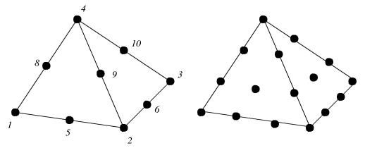
Figure 23: The nodes for the quadratic and cubic elemental functions on the tetrahedron.

17.2The cube

The canonical cube is defined as

{(ξ, η, ζ) : −1 ≤ ξ, η, ζ ≤ 1}.

The elemental function for the node (ijk) is written as the direct product of the one-dimensional linear functions:

Nijk = Ni(ξ)Nj(η)Nk(ζ).

18 The interpolation error

The estimation of the interpolation errors will be done in two steps:

•the interpolation error estimation with polynomials on the canonical element

•the recalculation of the interpolation errors from the canonical to the physical element.

67

Figure 24: The nodes for the tri-linear tri-quadratic elemental functions on the cube.

For the sake of simplicity, let us consider the two-dimensional case. We expand a function on the canonical element in terms of the elemental functions

Then the interpolation error on the canonical element is estimated with the following

Theorem 1: Let p be the maximal integer number, such that Eq.(55) is exact for any polynimial of the degree p. Then for the canonical element Ω0 there exists C > 0 such that

|u − U|s,Ω0 ≤ C|u|p+1,Ω0 ,

u Hp+1(Ω0), s = 0, 1...p + 1.

where |u|s,Ω0 stands for the Sobolev quasinorm.

68