

The di erence becomes especially pronounced for the higher order elements
in the three-dimensional space.
|
|
R2 |
|
R3 |
|
n |
Order |
Ntens |
Nopt |
Ntens |
Nopt |
1 |
1 |
1 |
1 |
1 |
1 |
2 |
3 |
4 |
4 |
8 |
5 |
3 |
5 |
9 |
7 |
27 |
14 |
4 |
7 |
16 |
12 |
64 |
30 |
Table 2: The number of nodes n for the one-dimensional formulas, the formula orders and the node number for the tensor-type Ntens and optimal Nopt formulas.
21.2The quadrature formulas for the triangles
For the low order quadrature formulas, it is possible to derive them with the undetermined coe cient approach. We assume that the formula can be written in the following way
Z Z
f(ξ, η)dξdη = W1f(ξ1, η1) + E.
Ω0
As the formula contains three coe cient, it can be exact for all linear functions. So we substitute the following functions
f(ξ, η) = [1, ξ, η]>,
and calculate the integrals
1 |
1−ξ |
1 |
dηdξ = |
|
1/2 |
= |
|
W1 |
|
. |
|
Z |
Z |
|
ξ |
1/6 |
W1 |
ξ1 |
|||||
|
η |
|
|
1/6 |
|
|
W1 |
η1 |
|
||
0 |
0 |
|
|
|
|
||||||
We can see now that the solution exists as we are able to find all undetermined coe cients: W1 = 1/2, ξ1 = η1 = 1/3. The corresponding quadrature formula is written as
Z Z
f(ξ, η)dξdη = 12f(1/3, 1/3) + O(f00).
Ω0
89

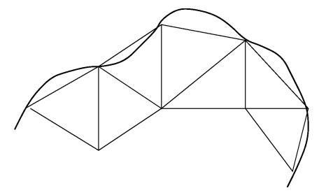
The quadrature formulas of the higher order are presented on figure (39) for the triangles and on figure (40) for the tetrahedrons.
Figure 39: The quadrature formulas for the triangles.
22The discretization and perturbation errors
We have already found that for the interpolation errors, the following theorem
is satisfied:
90

Figure 40: The quadrature formulas for the tetrahedrons.
Let Ω be divided into elements Ωe from the regular family. Let h be the longest side in the mesh. For the interpolation of the order p there exists a constant C > 0 (which is independent on u Hp+1(Ω) and the mesh) such that
|u − U|s ≤ Chp+1−s|u|p+1, s = 0, 1. |
(60) |
The convergence (60) is getting worse when the solution u is not smooth enough, see Lecture 6.
However, error estimation (60) does not take into account all possible errors in the FEM. Namely, it does not account for
•numerical integration errors,
•boundary condition approximation errors,
•boundary triangulation errors.
Let us discuss now the results which describe these kinds of errors.
91

22.1The numerical integration errors
We start from the initial variational problem
A(u, v) = (f, v) v H,
and apply the Galerkin method to this problem assuming the exact calculation of the integrals:
A(U, V ) = (f, V ) V HN
Now we will account for the approximate integration. This means that both the bilinear and linear forms are changed:
A (U , V ) = (f, V ) V HN
in the way we discussed above:
N |
N n |
X |
X X |
(f, V ) = (f, V )e, = |
WkV (xk, yk)f(xk, yk). |
e=1 |
e=1 k=1 |
For this problem, the following results can be proved.
Theorem 1. Let A(u, v) and A (U, V ) be the bilinear forms, the form A be the continuous form, and A be positively defined, i.e. there exist two constants
α and β such that
|
|
|A(u, v)| ≤ α||u||1||v||1, u, v H, |
|
|
|
|
|
||
|
|
A (U, U) ≥ β||U||12, U HN . |
|
|
|
|
|
||
Then |
|
|
|
|
|
|
|
|
|
|
|
||u − U ||1 ≤ C {||u − V ||1+ |
|
|
|
|
|
||
+ sup |
|
A(W, V ) − A (W, V )| |
+ sup |
|(f, W ) − (f, W ) | |
, |
|
V |
|
HN . |
|
|
||W ||1 |
|||||||
| |
||W ||1 |
|
|
|
|||||
One can see that this theorem gives us a possibility to separate two types of errors: the interpolation errors with the exact integration described by
92

Eq.(60), and the errors erasing from the numerical integration. The numerical integration errors themselves are covered by the next theorem.
Theorem 2. Let J(ξ, η) |
be the Jacobian of the transformation from the |
(ξ, η) into (x, y) plane. Let |
h be the regular FEM family. Let det(J(ξ, η))Wx(ξ, η) |
and det(J(ξ, η))Wy(ξ, η) be the piecewise polynomials of the degree less or equal to r1, and det(J(ξ, η))W (ξ, η) be the piecewise polynomials of the degree less or equal to r0. Then:
1. If the quadrature formula in (ξ, η) is exact for polynomials of the r1 + r degree, then
|A(W, V ) − A (W, V )| |
≤ |
Chr+1 |
|| |
V |
||r+2 |
, V, W |
|
HN . |
||W ||1 |
|
|
|
|
2. If the quadrature formula in (ξ, η) is exact for polynomials of the r1 +r −1 degree, then
|(f, W ) − (f, W ) | |
≤ |
Chr+1 |
f |
, |
|
W |
|
HN . |
|
||W ||1 |
|||||||||
|
|| ||r+1 |
|
|
|
Here we have the estimation of the numerical integration inaccuracy for both bilinear and linear forms. Let us consider two examples of the application of theorem 2.
Example 1. Let the coordinate transformation be the linear one. Then the Jacobian determinant det(J(ξ, η)) is a constant. Let also the space HN consist of the piecewise polynomials of the degree p (i.e. we consider the FEM of the order p with the linear coordinate transformation). For this case, we can see that r1 = p − 1, r0 = p. According to the interpolation theorem, we find
||u − V ||1 = O(hp)
Let now assume that we use the quadrature formula of the order ρ. Then ρ = r1 + r and ρ = r0 + r − 1, and we find
r = ρ − p + 1.
Applying Theorem 2, we find:
|A(W, V ) − A (W, V )| ≤ Chρ−p+2||V ||ρ−p+3.
||W ||1
93

|(f, W ) − (f, W ) | ≤ Chρ−p+2||f||ρ−p+2.
||W ||1
Depending on the values of p and ρ, we can have the di erent cases:
1. If ρ = 2(p −1) then r = p −1. All errors have the same order with respect to h:
||u − U ||1 = O(hp).
This situation is optimal, as we acquire the best convergence speed possible, but we do not spend excessive e ort for the numerical integration.
2. If ρ > 2(p − 1) then r > p − 1. The interpolation error is the main error:
||u − U ||1 = O(hp).
The integration error has a higher order with respect to h and does not contribute to the last estimation. Again, we have the best convergence speed possible, but the additional numerical integration e ort may be meaningless. 3. If ρ < 2(p − 1) then r < p − 1. The integration error is the main error:
||u − U ||1 = O(hρ−p+2).
In this case, we do reach the convergence speed which is possible for the chosen FEM. Even worse, if ρ ≤ p − 2 (i.e. we use the low order quadrature formula for the higher order polynomials), the FEM approximation does not converge to the exact result when h → 0.
Example 2. Let us consider the isoparametric elements. For them, the degree of the coordinate transformations coincides with the order of the elemental functions. Then one can check that the optimal integration order
ρ is found as
ρ = 4(p − 1).
22.2The boundary condition approximation errors
Here we just present the basic result for this kind of errors. Namely, if the integration is exact, and there are no boundary triangulation errors, then for
94
the degree p polynomials one can find that
||u − U||1 ≤ hp||u||p+1 + hp+1/2||u||p+1 , |
(61) |
for the solution u Hp+1(Ω). If the boundary of the domain Ω is not smooth (e.g. it contains edges), then the solution may not belong to the space Hp+1(Ω), and estimation (61) is not valid.
22.3The boundary triangulation errors
Figure 41: The approximation of the domain boundary with polynomials.
The specific problem for this type of errors is due to the fact that the space of approximating functions do not necessarily belong to the full initial functional space. This requires a special consideration of the problem.
A few results are derived for this type of errors. For example, for the linear approximation
||u − U||1 = O(h),
while for the quadratic one
||u − U||1 = O(h3/2).
95
The detailed analysis shows that errors of this type are localized in a vicinity
∂Ω, while outside that vicinity they are not influenced by the boundary approximation.
Another known result is the following one: for the approximation with the degree p polynomials,
||u − U||1 = O(hp),
˜
if the distance between the exact ∂Ω and approximated ∂Ω boundaries is proportional to hp+1. Therefore, in order to reach the optimal convergence, we should approximate the boundary by the degree p polynomials. This means, that the optimal convergence near the domain boundary can be achieved with the isoparametric finite elements.
96
Lecture 9
A priori and a posteriori error estimations. Superconvergence. Adaptive solution
refinement. h-, p-, and hp-refinement.
23 A priori and a posteriori error estimations
For the error estimations in all branches of the numerical analysis including the FEM there widely use two types of methods: a priori and a posteriori methods. According to their names, a priori methods can give some information about the accuracy of the solution prior to the solution itself is actually computed. A posteriori methods require a solution (or, typically, few solutions) to be calculated, then they can measure its accuracy.
In the frame of the FEM, a priori error estimations are well-known. In the most regular cases, they can be described as
|u − U|s ≤ Chp+1−s|u|p+1, |
(62) |
s = 0, 1, u Hp+1(Ω),
where h is the maximal finite element volume. In Eq.(62), the approximation
U for the exact solution u is constructed in the domain Ω, and the error estimations are given for the solution and its derivatives. The advantage of these estimations is that we know them before any solution is constructed. On the other hand, we do not know as a rule the value of the constant C in the r.h.s. and the norm of the exact solution, and, therefore, cannot estimate the error quantitatively.
As we have already mentioned, a posteriori estimations employ already known approximate solutions in order to estimate errors quantitatively. One can find di erent a posteriori estimators, so it is worthwhile to formulate the requirements to get useful estimators. As a rule, the applicable estimator must
•give accurate error estimation for arbitrary meshes and polynomial degrees,
97
•be computationally e ective
•be able to work with di erent norms of the solution. The main types of a posteriori estimations are based on
•the extrapolation of the solutions,
•the calculation of the solution residuals,
•the solution recovery.
Let us analyze these estimators.
23.1Estimators based on the solution extrapolation
Space extrapolation
Let us construct two approximate solutions Uhp(x) and Uh/p 2(x), corresponding to the finite element volumes h and h/2. Then we assume that the error estimation in Eq.(62) is in fact exact:
u(x) − Uhp(x) = Cp+1hp+1 + O(hp+2) |
(63) |
|||||
|
h |
p+1 |
|
|||
u(x) − Uh/p 2(x) = Cp+1 |
|
|
|
+ O(hp+2) |
|
|
2 |
|
|||||
Substracting last equations from each other, we get |
|
|||||
Uh/p 2(x) − Uhp(x) = Cp+1hp+1(1 − |
1 |
) + O(hp+2). |
|
|||
|
|
|
||||
|
2p + 1 |
|
||||
Ignoring the higher order terms with respect to h, we find the error estimation
p |
|
Uh/p 2(x) − Uhp(x) |
|||
u(x) − Uh |
(x) ≈ |
1 |
− |
1/2p+1 |
. |
|
|
|
|
|
|
So we get the approximate expression for the solution Uhp(x) inaccuracy in terms of the solution itself and another solution calculated on the twice finer mesh. This approach to the error estimation construction is called Richardson’s extrapolation, or h-extrapolation.
98