Beginning Algorithms (2006)

Chapter 17

if (source.charAt(row - 1) != target.charAt(col – 1)) { cost = _costOfSubstitution;

}

return grid[row - 1][col - 1] + cost;

}

The method deleteCost() calculates the cost of deletion by adding the cumulative value from the cell directly above to the unit cost of deletion:

private int deleteCost(int[][] grid, int row, int col) { return grid[row - 1][col] + _costOfDeletion;

}

Lastly, insertCost() calculates the cost of insertion. This time, you add the cumulative value from the cell directly to the left of the unit cost of insertion and return that to the caller:

private int insertCost(int[][] grid, int row, int col) { return grid[row][col - 1] + _costOfInsertion;

}

The method minimumCost calculates the cost of each of the three operations and passes these to min() — a convenience method for finding the minimum of three values:

private int minimumCost(CharSequence source, CharSequence target, int[][] grid, int row, int col) {

return min(

substitutionCost(source, target, grid, row, col), deleteCost(grid, row, col),

insertCost(grid, row, col)

);

}

private static int min(int a, int b, int c) { return Math.min(a, Math.min(b, c));

}

Now we can get into the algorithm proper. For this, you defined the method calculate(), which takes two strings — a source and a target — and returns the edit distance between them.

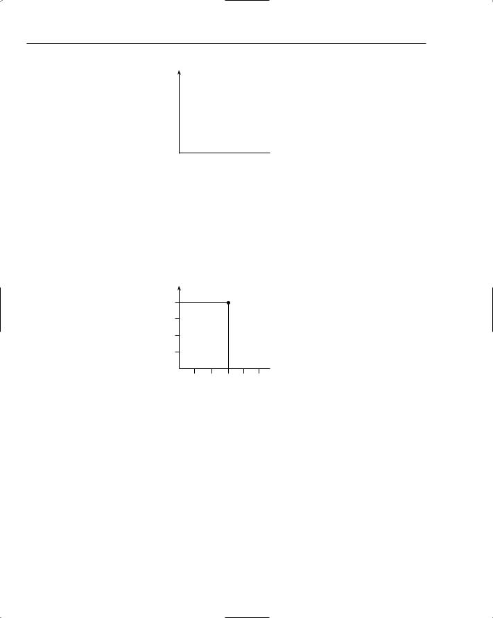
The method starts off by initializing a grid with enough rows and columns to accommodate the calculation, and the top-left cell of the grid is initialized to 0. Then, each column in the first row and each row in the first column are initialized, with the resulting grid looking something like the one shown in Figure 17-11.

Next, you iterate over each combination of source and target character, calculating the minimum cost and storing it in the appropriate cell. Eventually, you finish processing all character combinations, at which point you can select the value from the cell at the very bottom-right of the grid (as we did in Figure 17-13) and return that to the caller as the minimum distance:

public int calculate(CharSequence source, CharSequence target) { assert source != null : “source can’t be null”;

434

String Matching

assert target != null : “target can’t be null”;

int sourceLength = source.length(); int targetLength = target.length();

int[][] grid = new int[sourceLength + 1][targetLength + 1];

grid[0][0] = 0;

for (int row = 1; row <= sourceLength; ++row) { grid[row][0] = row;

}

for (int col = 1; col <= targetLength; ++col) { grid[0][col] = col;

}

for (int row = 1; row <= sourceLength; ++row) { for (int col = 1; col <= targetLength; ++col) {

grid[row][col] = minimumCost(source, target, grid, row, col);

}

}

return grid[sourceLength][targetLength];

}

Summar y

So-called phonetic coders such as Soundex can efficiently find similar sounding words.

Soundex values are often used to find duplicate entries and misspelled names in databases.

Soundex calculates a four-character code in O(N) time.

Levenshtein word distance calculates the number of operations necessary to transform one word into another — the smaller the distance, the more similar the words.

The Levenshtein algorithm forms the basis for spell-checkers, DNA searches, plagiarism detection, and other applications.

The Levenshtein algorithm runs in the time and space complexity of O(MN).

435

18

Computational Geometr y

This chapter gives you a taste of a fascinating area of algorithm design known as computational geometry. This topic could fill dozens of books on its own, so we will only be scratching the surface here. If you want to know more, check out the references or search the Internet for more material.

Computational geometry is one of the foundations of computer graphics, so if you intend to pursue an interest in developing software for games or other graphical areas, you’ll need a solid understanding of computational geometry.

All topics covered in this chapter are limited to two-dimensional geometry. You will need to grasp the concepts in two dimensions before understanding three dimensions, a topic beyond the scope of this chapter. There are many excellent books that specialize in the explanation of the algorithms used in three-dimensional graphics. Check the references section in Appendix A or a good computer bookstore.

This chapter discusses the following topics:

A quick geometry refresher

Finding the intersection point of two straight lines

Finding the closest pair of points among a large set of scattered points

A Quick Geometr y Refresher

This section saves you the trouble of digging out your high school mathematics textbook by quickly recapping some of the concepts you’ll need to understand to make sense of the rest of the chapter.

Coordinates and Points

Two-dimensional spatial concepts are usually described using an x-y coordinate system. This system is represented by two straight lines called axes that are perpendicular to each other, as shown in Figure 18-1.

Chapter 18

Y axis

X axis

Figure 18-1: The x-y coordinate system is made up of two axes.

The horizontal axis is called the x axis and the vertical axis is called the y axis. Positions along the x axis are numbered from left to right with increasing values. Positions on the y axis have values that increase as they move upwards.

A point is a position in two-dimensional space that is defined by two numbers in the form (x, y), where x is the value on the x axis directly below the point, and y is the value on the y axis directly to the left of the point. For example, Figure 18-2 shows the point (3, 4) in the coordinate system.

Y axis

(3,4)

4

3

2

1

X axis

Figure 18-2: The point (3, 4) in the x-y coordinate system.

The x-y coordinate system also extends to the left and below the axes shown. Positions along these ends of the axes are defined by negative coordinates, as shown in Figure 18-3, which has points plotted in various regions.

Lines

A line is simply a straight path between two points. The two end-points are all that is needed to define a line. From that, you can determine its length, its slope, and other interesting things, but we’ll get to that soon enough. Figure 18-4 shows the line (1, 1) – (5, 4).

438

Computational Geometry

-3

(-2,-3)

-4 -5

Figure 18-3: Coordinates can also be negative on both the x and y axes.

4

3

2

1

Figure 18-4: A line in the x-y coordinate system.

Triangles

We won’t insult you by telling you what a triangle is (apologies if we did so when describing what a line is in the preceding section). You are mainly interested in right-angled triangles in this chapter; they’re the ones with one 90-degree angle, as shown in Figure 18-5.

The best thing about right-angled triangles is that if you know the lengths of two of the sides, you can use Pythagoras’ theorem to figure out the length of the third side. In Figure 18-5, the sides are labeled a, b, and c. Pythagoras’ theorem states that

a2 + b2 = c2

as long as c refers to the longest side, or hypotenuse. The usual example is a triangle like the one shown in Figure 18-6, with side lengths of 3, 4, and 5.

439

Chapter 18

c

a

b

Figure 18-5: A right-angled triangle.

5

3

4

Figure 18-6: A right-angled triangle with side lengths specified.

Looking at the figure, it’s easy to see that . . .

32 + 42 = 52

Or . . .

9 + 16 = 25

That’s about all the background you need before you explore the first computational geometry problem: determining where two lines intersect.

Finding the Intersection of Two Lines

This section walks you through a computational geometry problem that finds the point where two lines intersect. Figure 18-7 shows two lines intersecting at the point marked P.

If all you know are the four points that define the end-points of the two lines, how do you figure out where (and if) the two lines intersect? The first thing you need to be comfortable with is the algebraic formula for a line, which is

y = mx + b

where y and x are the coordinates you’re already familiar with, m is the slope of the line, and b is the point at which the line cuts the y axis. Don’t worry, we’ll explain these concepts next.

440

Computational Geometry

Figure 18-7: Two intersecting lines.

Slope

The slope of a line is simply how steep it is. You use a simple method to describe this, depicted in Figure 18-8.

4

3

rise

2

1

travel

Figure 18-8: The slope of a line expressed as the ratio of rise to travel.

The rise is the vertical distance (amount of y axis) covered by the line. The travel is the horizontal distance (amount of x axis) covered by the line. Finally, the slope is the ratio of rise to travel. For example, a line that has the same rise as travel has a slope of 1, as shown in Figure 18-9.

(4,4)

4

3

Slope = 1

Rise = 3

2

1

Figure 18-9: A line with a slope of 1.

441

Chapter 18

Slopes can be negative. Figure 18-10 shows a line with a slope of –2, as its rise (or fall!) from the first point to the second point is downward, or negative, and is twice as large as its travel.

Figure 18-10: A line with a negative slope.

There are a couple of special cases to note also. Horizontal lines have a slope of zero, because no matter how large their travel, their rise is zero. More of an issue is the vertical line, which has a travel of zero no matter how much rise it has. Recall that slope is the ratio of rise to travel, which means you divide rise by travel to derive the slope. Of course, dividing by zero is impossible, so vertical lines have an infinite slope, which is of little meaning to a computer. You have to be very careful when coding to avoid issues with vertical lines, as you will see later.

Crossing the y Axis

Lines that have the same slope as each other are parallel. Two lines with the same slope differ in the point at which they cross the y axis (unless they are vertical, but don’t worry about that for now). Figure 18-11 shows two parallel lines with a slope of 0.5 that cross the y axis at two different points.

Figure 18-11: A pair of parallel lines.

Note how the higher line crosses the y axis at the y value of 2, so its formula is

y = 0.5x + 2

442

Computational Geometry

The lower line crosses the y axis at the y value –1, so its formula is

y = 0.5x – 1

Finding the Intersection Point

You now have enough background to work through an example of finding the intersection point of two lines. Use Figure 18-12 for this purpose.

Figure 18-12: A sample pair of intersecting lines.

The trick is that the coordinates of the point of intersection will make sense in either of the formulas for the two lines. In other words, if the formula for the first line is as follows:

y = mx + b

And the formula for the second line is as follows:

y = nx + c

To find the point of intersection, use the following:

mx + b = nx +c

Rearrange that as follows:

mx – nx = c – b

Rearrange again:

x = (c – b) / (m – n)

443