Beginning Algorithms (2006)

Chapter 14

airpost alright apricot

Pretty handy the next time you’re stuck while trying to solve a crossword or even when playing Scrabble.

Summar y

This chapter demonstrated the following about ternary search trees and associated behavior:

They are most useful for storing strings.

Aside from a regular lookup, they can be used for prefix searching.

They can also be used for pattern matching, such as for solving crossword puzzles.

They are like binary search trees with an extra child node.

Instead of holding the entire word, nodes contain one letter each.

Like binary search trees, ternary search trees can become unbalanced.

They are generally more time efficient than binary search trees, performing on average fewer numbers of character comparisons.

Exercise

1.Create an iterative form of search().

374

Chapter 15

You already know that a binary search tree is composed of individual nodes, so maybe you could try reading and writing the nodes individually instead of all in one go. While this sounds like a good idea at first, in practice it turns out to be rather less than ideal. Recall that even in a perfectly balanced binary search tree, the average number of nodes traversed to find a search key will be O(log N). For our imaginary database containing a million records, this would therefore be log2 1,000,000 = 20. This is fine for in-memory operations for which the cost of accessing a node is very small, but not so great when it means performing 20 disk reads. Even though each node is quite small — in our example, only 26 or so bytes — data is stored on disks in much larger blocks, sometimes referred to as pages, so the cost of reading one node is no more or less expensive than reading, for example, 20 nodes. That’s great, you say, you only need to read 20 nodes, so why not just read them all at once?

The problem is that given the way a binary search tree is built, especially if some kind of balancing is occurring, it’s highly unlikely that related nodes will be located anywhere near each other, let alone in the same sector. Even worse, not only will you incur the cost of making the 20 or so disk reads, known as transfer time, but before each disk read is performed, the heads on the disks need to be repositioned, known as seek time, and the disks must be rotated into position, known as latency. All of this adds up. Even if you employed some sophisticated caching mechanisms in order to reduce the number of physical I/Os performed, the overall performance would still be unacceptable. You clearly need something better than this.

B-Trees are specifically designed for managing indexes on secondary storage such as hard disks, compact discs, and so on, providing efficient insert, delete, and search operations.

There are many variations on the standard B-Tree, including B+Trees, B×Trees, and so on. All are designed to solve other aspects of searching on external storage. However, each of these variations has its roots in the basic B-Tree. For more information on B-Trees and their variations, see [Cormen, 2001], [Sedgewick, 2002], and [Folk, 1991].

Like binary search trees, B-Trees contain nodes. Unlike binary search trees, however, the nodes of a B-Tree contain not one, but multiple, keys, up to some defined maximum — usually determined by the size of a disk block. The keys in a node are stored in sorted order, with an associated child node holding keys that sort lower than it — every nonleaf node containing k keys must have k+1 children.

Figure 15-1 shows a B-Tree holding the keys A through K. Each node holds at most three keys. In this example, the root node is only holding two keys — D and H — and has three children. The leftmost child holds all keys that sort lower than D. The middle child holds all keys that sort between D and H. The rightmost child holds all other keys greater than H.

D H

A B C E F G I J K

Figure 15-1: A B-Tree with a maximum of three keys per node, holding the keys A through K.

Looking for a key in a B-Tree is similar to looking for a key in a binary search tree, but each node contains multiple keys. Therefore, instead of making a choice between two children, a B-Tree search must make a choice between multiple children.

376

B-Trees

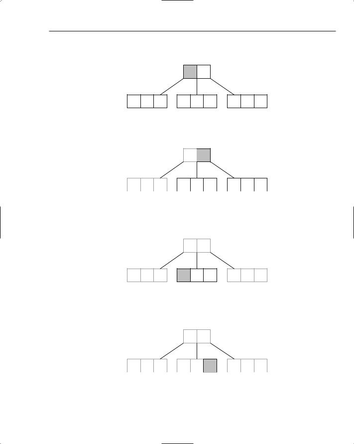
As an example, to search for the key G in the tree shown in Figure 15-1, you start at the root node. The search key, G, is first compared with D (see Figure 15-2).

D H

A B C E F G I J K

Figure 15-2: A search starts at the first key in the root node.

Because G sorts after D, the search continues to the next key, H (see Figure 15-3).

D H

Figure 15-3: The search continues at the next key in the node.

This time, the search key sorts before the current key in the node, so you follow the link to the left child (see Figure 15-4).

D H

Figure 15-4: The search key falls below the current key so the search continues by following the left child link.

This continues until eventually you find the key for which you are searching (see Figure 15-5).

Figure 15-5: The search ends with a match.

Even though the search performed five key comparisons, only two nodes were traversed in the process. Like a binary search tree, the number of nodes traversed is related to the height of the tree. However,

377

Chapter 15

because each node in a B-Tree contains multiple keys, the height of the tree remains much lower than in a comparable binary search tree, resulting in fewer node traversals and consequently fewer disk I/Os.

Going back to our original example, if we assume that our disk blocks hold 8,000 bytes each, this means that each node can contain around 8,000 / 26 = 300 or so keys. If you have a million keys, this translates into 1,000,000 / 300 = 3,333 nodes. You also know that, like a binary search tree, the height of a B-Tree is O(log N), where N is the number of nodes. Therefore, you can say that the number of nodes you would need to traverse to find any key would be in the order of log300 3,333 = 2. That’s an order of magnitude better than the binary search tree.

To insert a key into a B-Tree, start at the root and search all the way down until you reach a leaf node. Once the appropriate leaf node has been found, the new value is inserted in order. Figure 15-6 shows the B-Tree from Figure 15-1 after the key L has been inserted.

D H

Figure 15-6: Insertion always occurs at the leaf nodes.

Notice that the node into which the new key was inserted has now exceeded the maximum allowed — the maximum number of keys allowed in this example was set at three. When a node becomes “full,” it is split into two nodes, each containing half the keys from the original, as shown in Figure 15-7.

Figure 15-7: Nodes that become “full” are split in two.

Next, the “middle” key from the original node is then moved up to the parent and inserted in order with a reference to the newly created node. In this case, the J is pushed up and added after the H in the parent node, and references the node containing the K and L, as shown in Figure 15-8.

D H J

Figure 15-8: The middle key from the original node moves up the tree.

378

B-Trees

In this way, the tree spreads out, rather than increasing in height; B-Trees tend to be broader and shallower than most other tree structures, so the number of nodes traversed tends to be much smaller. In fact, the height of a B-Tree never increases until the root node becomes full and needs to be split.

Figure 15-9 shows the tree from Figure 15-8 after the keys M and N have been inserted. Once again, the node into which the keys have been added has become full, necessitating a split.

D H J

Figure 15-9: A leaf node requiring a split.

Once again, the node is split in two and the “middle” key — the L — is moved up to the root, as shown in Figure 15-10.

D H J L

Figure 15-10: The root node has become full.

This time, however, the root node has also become full — it contains more than three keys — and therefore needs to be split. Splitting a node usually pushes one of the keys into the parent node, but of course in this case it’s the root node and as such has no parent. Whenever the root node is split, a new node is created and becomes the new root.

Figure 15-11 shows the tree after the root node has been split and a new node is created above it, increasing the height of the tree. A new node containing the key H is created as the parent of the two nodes split from the original root node.

H

D J L

A B C E F G I K M N

Figure 15-11: Splitting the root node increases the height of the tree.

379

Chapter 15

Deletion from a B-Tree is rather more complicated than both search and insert as it involves the merging of nodes. For example, Figure 15-12 shows the tree after deleting the key K from the tree shown in Figure 15-11. This is no longer a valid B-Tree because there is no longer a middle child (between the keys

J and L). Recall that a nonleaf node with k keys must always have k+1 children.

Figure 15-12: Deleting the key K produces an invalid B-Tree.

To correct the structure, it is necessary to redistribute some of the keys among the children — in this case, the key J is pushed down to the node containing the single key I, shown in Figure 15-13.

Figure 15-13: Keys are redistributed among the children to correct the tree structure.

This is only the simplest situation. If, for example, the keys I and J were deleted, then the tree would look like the one shown in Figure 15-14.

Figure 15-14: Redistribution is required to correct the tree structure.

380

B-Trees

Again, a redistribution of keys is required to correct the imbalance in the tree. You can achieve this in several ways. No matter how the keys are redistributed, however, keys from parent nodes are merged with those of child nodes. At some point, the root node must be pulled down (or removed, for that matter). When this happens, the height of the tree is reduced by one.

For the purposes of this example, you’ll merge the L into its child and pull down the root node, H, as the parent (see Figure 15-15).

D H

Figure 15-15: The height of the tree drops whenever the root node is either merged into a child or deleted completely.

As you can see, deletion is a rather complicated process and involves many different scenarios. (For a more in-depth explanation, refer to [Cormen, 2001].)

Putting B-Trees into Practice

Now that you understand how B-Trees work and why they are useful, it’s time to try your hand at implementing one. As mentioned earlier, B-Trees are usually used as indexes, so in this simple example you’ll create an implementation of the Map interface from Chapter 13, based on a B-Tree. However, to avoid detracting from the underlying workings of the algorithms involved, the class you create will be purely in-memory, rather than on disk.

You’ll implement all the methods from the Map interface using your understanding of B-Trees as the basis of the underlying data structure. To this end, you’ll implement the get(), contains(), and set() methods based on the search and insertion algorithms discussed earlier. For the delete() method, however, you’re going to cheat a little. Because the algorithm for deleting from a B-Tree is extremely complicated — involving at least three different scenarios requiring entries to be redistributed among nodes — rather than actually delete the entries, you’ll instead simply mark them as deleted. While this does have the rather unfortunate side-effect that the B-Tree will never release any memory, it is sufficient for the purposes of this example. For a more detailed explanation of B-Tree deletion, see [Cormen, 2001].

In the next Try It Out section, you create the tests to ensure that your B-Tree map implementation works correctly.

Create the BTreeMapTest class as follows:

package com.wrox.algorithms.btrees;

import com.wrox.algorithms.maps.AbstractMapTestCase; import com.wrox.algorithms.maps.Map;

381

Chapter 15

import com.wrox.algorithms.sorting.NaturalComparator;

public class BTreeMapTest extends AbstractMapTestCase { protected Map createMap() {

return new BTreeMap(NaturalComparator.INSTANCE, 2);

}

}

How It Works

You already developed the test cases in Chapter 13, so all you needed to do was extend AbstractMapTestCase. The only other thing you need to do is implement the method createMap() and return an instance of the BTreeMap class. The BTreeMap constructor takes two parameters: a comparator for ordering the keys and the maximum number of keys per node. In this case, you force the number of keys per node to be as small as possible, ensuring the maximum number of nodes possible. Although this would seem to defeat the purpose of a B-Tree — the whole point being to keep the height and number of nodes as small as possible — by doing so in the test, you’ll ensure that all the special cases, such as leaf-node and root-node splitting, are exercised.

Tests in place, in the next Try It Out section you create the actual B-Tree map implementation.

Create the BTreeMap class as follows:

package com.wrox.algorithms.btrees;

import com.wrox.algorithms.iteration.Iterator; import com.wrox.algorithms.lists.ArrayList; import com.wrox.algorithms.lists.EmptyList; import com.wrox.algorithms.lists.List;

import com.wrox.algorithms.maps.DefaultEntry; import com.wrox.algorithms.maps.Map;

import com.wrox.algorithms.sorting.Comparator;

public class BTreeMap implements Map {

private static final int MIN_KEYS_PER_NODE = 2;

private final Comparator _comparator; private final int _maxKeysPerNode; private Node _root;

private int _size;

public BTreeMap(Comparator comparator, int maxKeysPerNode) { assert comparator != null : “comparator can’t be null”;

assert maxKeysPerNode >= MIN_KEYS_PER_NODE : “maxKeysPerNode can’t be < “ + MIN_KEYS_PER_NODE;

_comparator = comparator; _maxKeysPerNode = maxKeysPerNode; clear();

}

public Object get(Object key) {

382

B-Trees

Entry entry = _root.search(key);

return entry != null ? entry.getValue() : null;

}

public Object set(Object key, Object value) { Object oldValue = _root.set(key, value);

if (_root.isFull()) {

Node newRoot = new Node(false); _root.split(newRoot, 0);

_root = newRoot;

}

return oldValue;

}

public Object delete(Object key) { Entry entry = _root.search(key); if (entry == null) {

return null;

}

entry.setDeleted(true); --_size;

return entry.setValue(null);

}

public boolean contains(Object key) { return _root.search(key) != null;

}

public void clear() { _root = new Node(true); _size = 0;

}

public int size() { return _size;

}

public boolean isEmpty() { return size() == 0;

}

public Iterator iterator() {

List list = new ArrayList(_size);

_root.traverse(list);

return list.iterator();

}

private final class Node {

383