Advanced Wireless Networks - 4G Technologies

108 ADAPTIVE AND RECONFIGURABLE LINK LAYER

4.1.4.1 Net bit rate

The error rate used for expressing QoS requirements is usually the packet error rate (PER) since it is closer to the user’s perception of quality. At the link layer, a packet is considered valid if no error is present or all errors have been corrected. In our model, the correction capability of the code is included in its coding gain, therefore, for the packet to be valid, no residual error is allowed. The packet error rate pE is therefore given by:

where pe(γ ) is the bit error rate of the uncoded system, Gc(γ ) is the coding gain, γ is the SINR per bit, and Lp is the packet length in bits. Any channel coding scheme can be included in this model provided that its performance is summarized in the coding gain curve, Gc(γ ). In Equation (4.7), errors in the header and in the payload are assumed equiprobable. In reality, errors in the header are more critical because they may cause erroneous addressing and insertion errors. If distinct channel coding schemes are adopted for the two parts, with a stronger code for the header, the probability of a novalid packet is pE = 1 − (1 − pE,h)

(1 − pE,i ) where the probabilities of erroneous header and payload are computed separately as pE,h = 1 − {1 − pe [γ Gc(γ )]}Lh and pE,i = 1 − {1 − pe [γ Gc(γ )]}Li , respectively.

Besides of its advantages in achieving reliable transfer of information, channel coding protection implies a loss in capacity due to the introduced redundancy. Moreover, each protocol layer adds its own header to the packet as it is proceeding downwards through the protocol stack. We assume in the following that the same channel coding scheme is applied to both header and payload. The generalization when distinct schemes are adopted is straightforward. The header efficiency is defined as the ratio between the payload size and the total packet size without redundancy (i.e. header and payload together, Ld = Li + Lh): ηh = Li /Ld. The channel coding efficiency depends on the added redundancy and is represented by its code rate ηc = Ld/(Ld + Lo). Since the packet size after channel coding and packetization can be written as Lp = Li + Lh + Lo = Li /(ηhηc), the bit rate for a given PHY mode (still including residual errors) can be written as

where ki is the number of bits per symbol of the ith mode modulation scheme, and Ts is the symbol duration.

4.1.5 Link service rate with exact mode selection

The link service capacity is the rate at which error-free information units are transmitted through the channel and is referred to as ‘goodput’. It is a function of the gross bit rate or throughput, which includes the corrupted information units, r, and the residual error rate after correction, e. By using a similar expression for the link service rate as given in Kim and Li [27] for ideal systems with fixed PHY, and extending it to time-varying systems, the goodput at a given instant t can be expressed as

In Equation (4.9), r(t) is the gross channel transmission rate, or throughput, which depends on modulation constellation size, code rate, overheads, etc., and e(t) is the residual

error rate, which depends essentially on modulation scheme, channel coding gain, diversity combining methods, and physical channel conditions. The residual error rate after reassembling e has the same value of the packet error rate defined in Equation (4.7) i.e. e = pE.

We extend further Equation (4.9) to adaptive systems. In adaptive systems the transceiver configuration settings change in time depending on the channel state at time t, denoted by S(t) = i or Si . The PHY mode ideally associated with each region and used at time t is denoted with M(t) = i or Mi . To simplify notation, whenever possible we drop the dependence on time t. In presence of ideal link adaptation, the service capacity is obtained averaging across all the modes, resulting in

where the subscript i denotes the mode, M is the number of implemented modes, and πi is the probability of the channel being in state i and using the ith mode.

4.1.5.1 Model of impairments

In Equation (4.10), the service capacities for all modes can be represented by a vector because the effective and chosen states are assumed to coincide. In case of erroneous mode selection, the gross bit rate depends on the used mode whereas the error rate depends on both the used mode and the effective state. Hence, in the presence of imperfections the two contributions must be separated. In the sequel, we will use the following notation.

goodput matrix Y = {yi j } RM×M includes the effects of errors due to corruption in the

channel for each PHY mode and each state, and expresses the useful bit rate normalized to

.

the transmit rate in each mode. The generic element of matrix Y is defined as yi j = 1 − ei j ,

CTMC. The mode selection is made by the adaptation algorithm based on an estimated channel conditions. If the adaptive system rapidly follows without errors the channel state, the average goodput, Equation (4.10), is expressed with the new notation by:

where = diag(π ) is.the diagonal matrix having as diagonal elements the elements of

vector π , and diag(A) = [aii ] is the operator that extracts the vector of diagonal elements of

.

matrix A: diag(A) = (A I)u, where I is the identity matrix, u is the unity vector having all elements 1, and is the Hadamard–Schur product.

represent either the quality metric region or the mode itself. After the estimation delay, the mode, subject to errors in the feedback channel, is transmitted and M(t + τe) = i is acquired at the transmitter (or at the receiver, in the open loop case). This mode is used for transmission (Figure 4.2; or reception, Figure 4.3). In the mean time, the effective channel quality metric falls in general in a new region, S(t + τe) = j, due to possible channel state transitions during the estimation delay τe. The model described here is unaffected whether estimator and mode selector are implemented at transmitter or receiver side, provided that proper values are given to related quantities. For example, in the open loop case, errors on the control message sent to the receiver through a separate channel are modeled with the feedback error. The final effect of the entire process is that in general mode Mi is used at transmission time, when the channel is in effective state Sj . According to the notation above, the probability of this event can be written as P(Mi , Mh , Sk , Sj ). Because the estimation process and the channel process are clearly independent, and assuming that the feedback channel is independent of the direct channel, we can write

P(Mh , Sk , Mi , Sj ) = P(Mh , Sk )P(Mi , Sj |Mh , Sk )

= P(Mh , Sk )P(Mi |Mh , Sk )P(Sj |Mi , Mh , Sk )

(4.13)

= P(Mh , Sk )P(Mi |Mh )P(Sj |Sk )

= P(Sk )P(Mh |Sk )P(Mi |Mh )P(Sj |Sk ).

The three last terms in Equation (4.13) are treated separately in the sequel and their effect on the goodput is then combined by averaging independently the appropriate expressions.

4.1.7 Estimation process and estimate error

In the absence of estimation delay and feedback errors, a possibly erroneous estimate of the metric at time t is used to choose the mode at time t, i.e. γˆ (t) → M(t). The mode estimation probability matrix H(e) = {h(e)hk } RM×M models the effects of the imperfections in the estimation process due to noise. Its generic element h(e)hk represents the probability of selecting mode Mh when the true channel is in state Sk at estimation time:

Equation (4.14) represents the second term in Equation (4.13).

4.1.8 Channel process and estimation delay

Now we study the probability that the true state has changed during the delay τe. Consider the presence of estimation delay and absence of estimate error and feedback errors. In other

words, the mode at time t + τe is chosen depending on the exact estimate of the metric at time t, i.e. γ (t) → M(t + τe). The delayed channel transition matrix H(d) = {h(d)k j } RM×M

models the effects of estimation delay. Its generic element h(d)k j represents the probability that given the true channel was in state k at estimation time, at transmission time the channel is in state j:

Equation (4.15) represents the last term in Equation (4.13).

¯ r corresponds to the average goodput of a system adopting an hypothetical set of PHY

R

modes all having unitary transmission rate. The use of this quantity will be elaborated later. In the ideal case of perfect link adaptation, the channel quality metric is estimated without errors, tracked without delay, and communicated to the transmitter without errors, i.e. H(e) = H(d) = H(f) = I, Ω reduces to the identity matrix, and we have Θ = Π. As a result, under the assumptions defined above, the definition of average goodput given in Equations (4.17) and (4.18) reduces to the one of the ideal case, Equations (4.11) and (4.12). Single PHY mode systems are considered in this model as a special case with errorless feedback channel, H(f) = I, instantaneous estimation, H(d) = I, and static mode selection leading to a matrix H(e) having as nonzero elements all 1 in the ith row, if mode Mi is implemented in the system: h(hke) = δhi δkk , where δi j is the Kronecker delta.

4.1.10.1 System performance

For illustration purposes, we apply the above analysis tool to the study of a sample system and investigate its sensitivity to some imperfection or implementation constraints.

4.1.10.2 System parameters

The PHY modes include a no-transmission mode for values of the signal quality that do not comply with minimum service requirements. The modulation schemes used in the numerical analysis are BPSK, QPSK, 8QAM and 16QAM. The channel coding scheme used is the half rate convolutional code having generator polynomials g0 = 1338 and g1 = 1718, and constraint length K = 7. Coding gain curves for the half rate and punctured versions of that mother code, having ηc = 2/3 and ηc = 3/4, are obtained from standard sources [28, 29]. The minimum signal to interference-plus-noise ratio for the coded system, γmin, is obtained from BERmax = BER γmin , knowing the coding gain for the given channel coding scheme:

γmin = γmin/Gc. Inverses of the BER of all schemes can be efficiently obtained from the approximated parametric function BER γ , valid for all schemes [25], or by numerical

inversion of exact expressions [30]. In the system used for numerical analysis, switching thresholds are obtained from the required PER for a packet length of 2048 b.

We assume Ricean fading process [31]. The expression for the LCR for the case of a line- of-sight component with zero Doppler frequency, uncorrelated Gaussian noise components, and Jakes-shaped Doppler power spectral density or isotropic scattering can be found in [32, 33]. Under the assumptions above, and using the corresponding LCR, expressions (4.1) and (4.2) can be written as

where fmax is the maximum Doppler frequency, σ0 is the standard deviation of the quadrature Gaussian components, pξ (ξk ; K f , σ0) is the value of the PDF of the Ricean distribution having Rice factor Kf at signal level ξk , and Pξ (ξk , ξk+1; K f , σ0) is the difference of the Rice cumulative distribution function (CDF) at points ξk+1 and ξk .

114 ADAPTIVE AND RECONFIGURABLE LINK LAYER

Table 4.1 Channel model parameters

State probabilities, level crossing rates downwards and upwards, and birth and death rates for the CTMC with five states used in the examples.

4.1.10.3 Channel model statistics

Parameters of the channel model for the example system are given in Table 4.1. Match of the statistics of the channel model is verified by comparing [34] the histogram obtained by simulation of the CTMC with the theoretical solution of the CTMC and with the theoretical PDF of the underlying fading process.

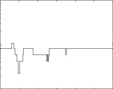
Figure 4.5 shows a snapshot of the time series obtained by simulations with above CTMC model with fmax = 300 Hz. It can be seen that very large changes in the metric (about one order of magnitude) occur in less than 1 ms around 3.5 ms, very rapid changes occur around 7 ms, and finally relatively long periods with steady values are seen on the right-hand side of the diagram. The system with fmax = 1 Hz simulated over 50 000 values, corresponding to a simulated time of tsim ≈ 4.6 h, exhibits τit,min ≈ 6.2 μs and τit,max ≈ 5.5 s as minimum and maximum of the inter-transition time, which depends on both the Doppler frequency of the fading process and the size of the signal quality regions.

4.1.11 Sensitivity of state probabilities to hysteresis region width

Consider the probability of staying in region Sk , πk . The kth state is entered by crossing levels γk + ϕk+ or γk−1 − ϕk−−1, when entering from below and above, respectively. This implies that in this case the actual width of the region is narrowed. Similarly, the state is left by crossing levels γk − ϕk− or γk−1 + ϕk+−1, when going below and above, respectively, and the actual width is now broadened. Although the ingress rate roughly equals the egress rate, as it can be seen in Table 4.1, the impact of hysteresis also depends on the state probabilities. In fact, the state probabilities after introducing the hysteresis can be written as:

i

(CDFi,±) is the half-width of the hysteresis region i at upper (+) and lower (−) side, respectively. In case of equal and symmetric hysteresis regions and neglecting higher order infinitesimals, we have

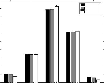
Figure 4.6 shows the sensitivity of state probabilities to CDF in this latter case, with regions defined as in Equation (4.6). For larger values of CDF, states with larger probability, the

116 ADAPTIVE AND RECONFIGURABLE LINK LAYER

Figure 4.6 Sensitivity of state probabilities to CDF. Up to about CDF = 10−3, state probabilities are unaffected. For larger values of CDF, states with large probability, the central ones in our case, have their probability further increased by the introduction of hysteresis. Bars are simulated values, whereas points are the theoretical values given by Equation (4.23).

In Equation (4.24) erfc(g) is the error function complement, σe is the standard deviation of

the estimation error, ¯k is the nominal value of the metric in the kth interval Sk , and inf(ξh )

ξ

and sup(ξh ) are the lower and upper boundaries, respectively, of interval Sh . Figure 4.7 shows the comparison of simulation and theoretical results for the sensitivity of the average

goodput ¯ c on estimate errors, under the assumptions given above in the non-coherent case,

R

assuming absence of estimation delay and error-free feedback channel.

4.1.12.1 Channel process and estimation delay

The variability in time of the quality metric depends on both the fading characteristics (coherence time) and the width of the state regions and is expressed by the inter-transition time, i.e. the time between state changes. In order to simplify the analysis, we assume that the estimation delay is negligible compared with the minimum inter-transition time. For our analysis it is sufficient to assume that i [0, M − 1] λi τe = qi,i+1τe = 1 and μi τe = qi,i−1τe = 1, where M is the cardinality of sets of PHY modes and quality regions. For the Poisson process, the reciprocal of the transition rate is the mean inter-transition time. The previous constraint states basically that the estimation delay should be much smaller than the mean inter-transition time.

Variance of estimation error, s 2e

Figure 4.7 Sensitivity of average goodput to variance of channel estimation error. Average

goodput ¯ c (solid line), scalar normalized average goodput ¯ r (dashed line),

R R and simulations (crosses).

Under the previous assumptions, at most one state change can occur during τe, and the probability of channel state transition can be written as:

It is straightforward to see that

where Q is the rate matrix of the CTMC and I is the identity matrix. In particular, in case of instantaneous channel estimation, matrix H(d) reduces to the identity matrix. The probability of no transition from the ith state is 1 − (λi + μi )τe. This term is null for τe = 1/(λi + μi ). Therefore, the quantity

has the meaning of coherence time in our model. Considering the case of perfect estimation and errorless feedback channel, and under the previous assumptions for the estimation delay model, the average goodput is expressed by: