808 Part VII Animation

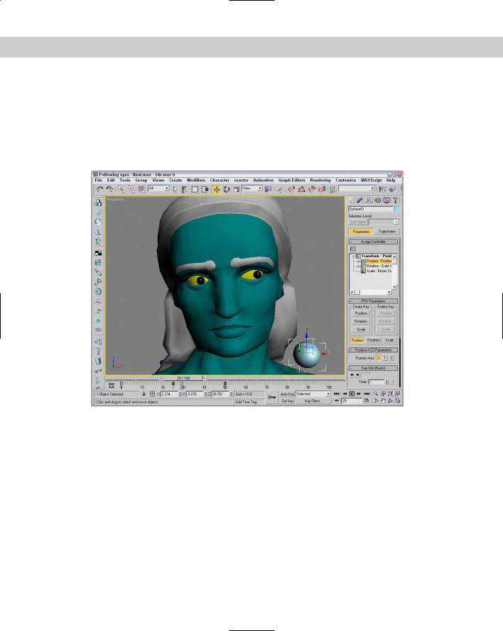
Then click the Debug button. The Expression Debug window appears, in which you can see the variable values change as items in the scene change. With the expression complete, you can drag the Time Slider back and forth and watch the pupil follow the ball from side to side. If you’re happy with the motion, click the Evaluate button and then the Close button to exit the interface.

This is a simple example, but it demonstrates what is possible. Figure 32-7 shows the resulting face.

Figure 32-7: The Expression controller was used to animate the eye’s following the ball in this example.

Understanding Expression Elements

The key to making the Expression controller work is building expressions. Before you can build expressions, you need to understand the various elements that make up an expression. Expressions can consist of variables (including predefined variables), operators, and functions, so we start by explaining these. It is also important to understand what the expression will return and the various return types.

Predefined variables

Max includes several predefined variables that have constant values. These predefined variables are defined in Table 32-1. They are case sensitive and must be typed exactly as they appear in the Syntax column.

Table 32-1: Predefined Variables

In addition to these predefined variables, you can choose your own variables to use. These variables cannot contain spaces, and each variable must begin with a letter. After a variable is defined, you can assign it a constant value or have it pick up its value from a controller track.

Operators

An operator is the part of an expression that tells how to deal with the variables. One example of an operator is addition: It tells you to add a value to another value. These operators can be grouped as basic operators, which include the standard math functions such as addition and multiplication; logical operators, which compare two values and return a true or false result; and vector operators, which enable mathematical functions between vectors. Tables 32-2 through 32-4 identify the operators that are in each of these groups.

Tip Although it isn’t required, scalar variables are typically lowercase and vector variables are uppercase.

Table 32-2: Basic Operators

810 Part VII Animation

Table 32-3: Logical Operators

Table 32-4: Vector Operators

The order in which the operators are applied is called operator precedence. The first equations to be calculated are the expressions contained inside of parentheses. If you’re in doubt about which expression gets evaluated first, place each expression in separate parentheses. For example, the expression (2 + 3) * 4 equals 20 and 2 + (3 * 4) equals 14. If the equation doesn’t contain any parentheses and only simple operators, then the precedence is from left to right with multiplication and division coming before addition and subtraction.

Functions

Functions are like mini-expressions that are given a parameter and return a value. For example, the trigonometric function for sine looks like this:

Sin()

It takes an angle, which is entered within the parentheses, and returns a sine value. For example, if you open the Expression Controller dialog box and enter the expression

Sin(45)

Table 32-5: Expression Functions

Continued

812 Part VII Animation

Table 32-5 (continued)

Return types

The return type can be a number (called a scalar), a collection of coordinates (called a vector), or a collection of color values (called a Point3). Scalars are used to control parameter values, vectors define actual coordinates in space, and the Point3 return type defines colors. Each of these types has its own format that you need to know before you can use it in an expression.

Scalar return type

A scalar value is a single value typically used for an object parameter, such as a sphere’s radius or the length of a Box object. This is used for tracks that have the Float Expression controller applied. Any resulting value from the expression is passed back to the assigned parameter. Scalars have no special format — only the number.

Vector return type

If a transform such as position is assigned, the Expression pane shows three values separated by commas and surrounded by brackets. These three values represent a vector, and each value is a different positional axis. You can refer to an individual axis value by placing a dot and the axis after the variable name. For example, if a vector variable named boxPosition exists, you can refer to the X-axis position component with the variable boxPosition.x. Component values are actually scalars.

Point3 return type

Materials work with yet another return type called a Point3. This type includes three numbers separated by commas and surrounded by brackets. Each of these values, which can range between 0 and 255, represents the amount of red, green, or blue in a color.

Note Any value that is out of range is automatically set to its nearest acceptable value. For example, if your expression returns a value of 500 for the green component, the color is shown as if green were simply 255.

Sample expressions

If you scan through your old physics and math books, you can find plenty of equations that you can use to create expressions. Following are some sample motions and their respective expressions.

For example, if the sphere object has the Float Expression controller applied to its Radius track, then a simple expression for increasing the radius from an initial radius value as the frame number increases would look like this:

initialRadius + F

You can use the trigonometric functions to produce a smooth curve from 0 to 360. Using the Sine function, you can cause the sphere’s radius to increase to a maximum value of 50 and then decrease to its original radius. The expression would look like this:

50 * sin(360*NT)

To make our sphere example move in a zigzag path, we can use the modulus function. This causes the position to increase slowly to a value and then reset. The expression looks like this:

[0, 10*mod(F,20), 10*F]

You can use the square root function to simulate ease in and ease out curves, causing the object to accelerate into or from a point. The expression would look like this:

[100*sqrt(NT*200), 10, 10]

Building complex expressions takes a little bit of math to accomplish, but it isn’t difficult to do and the more experience you get with expressions, the easier it becomes. To help get you started, Table 32-6 includes several prebuilt expressions that can be entered into the Expression Controller Interface to get certain motions.

Table 32-6: Sample Expressions

Continued