Wypych Handbook of Solvents
.pdf36 |
Koichiro Nakanishi |
48V. Moliner, J. Andrés, A. Arnau, E. Silla and I. Tuñón, Chem. Phys., 206, 57-61 (1996); R. Moreno, E. Silla,
I.Tuñón and A. Arnau, Astrophysical J., 437, 532-539 (1994); A. Arnau, E. Silla and I. Tuñón, Astrophysical
J.Suppl. Ser., 88, 595-608 (1993); A. Arnau, E. Silla and I. Tuñón, Astrophysical J., 415, L151-L154 (1993).
49M. D. Newton, S. J. Ehrenson, J. Am. Chem. Soc., 93, 4971 (1971). G. Alagona, R. Cimiraglia, U. Lamanna, Theor. Chim. Acta, 29, 93 (1973). J. E: del Bene, M. J. Frisch, J. A. Pople, J. Phys. Chem., 89, 3669 (1985).
I.Tuñón, E. Silla, J. Bertrán, J. Phys. Chem., 97, 5547-5552 (1993).
50R. Car, M. Parrinello, Phys. Rev. Lett., 55, 2471 (1985).
51P. G. Jonsson and A. Kvick, Acta Crystallogr. B, 28, 1827 (1972).
52A. G. Csázár, Theochem., 346, 141-152 (1995).
53Y. Ding and K. Krogh-Jespersen, Chem. Phys. Lett., 199, 261-266 (1992).
54J. H. Jensen and M.S.J. Gordon, J. Am. Chem. Soc., 117, 8159-8170 (1995).
55F. R. Tortonda., J.L. Pascual-Ahuir, E. Silla, and I. Tuñón, Chem. Phys. Lett., 260, 21-26 (1996).
56T.N. Truong and E.V. Stefanovich, J. Chem. Phys., 103, 3710-3717 (1995).
57N. Okuyama-Yoshida et al., J. Phys. Chem. A, 102, 285-292 (1998).
58I. Tuñón, E. Silla, C. Millot, M. Martins-Costa and M.F. Ruiz-López, J. Phys. Chem. A, 102, 8673-8678 (1998).
59F. R. Tortonda, J.L. Pascual-Ahuir, E. Silla, I. Tuñón, and F.J. Ramírez, J. Chem. Phys., 109, 592-602 (1998).
60F.J. Ramírez, I. Tuñón, and E. Silla, J. Phys. Chem. B, 102, 6290-6298 (1998).
61I. Tuñón, E. Silla and J.L. Pascual-Ahuir, J. Am. Chem. Soc., 115, 2226 (1993).
62I. Tuñón, E. Silla and J. Tomasi, J. Phys. Chem., 96, 9043 (1992).
63K.A. Connors, Chemical Kinetics, VCH, New York, 1990, pp. 134-135.
64N. Menschutkin, Z. Phys. Chem., 6, 41 (1890); ibid., 34, 157 (1900).
65J. Andrés, S. Bohm, V. Moliner, E. Silla, and I. Tuñón, J. Phys. Chem., 98, 6955-6960 (1994).
66S. Swaminathan and K.V. Narayan, Chem. Rev., 71, 429 (1971).
67N.K. Chaudhuri and M. Gut, J. Am. Chem. Soc., 87, 3737 (1965).
68M. Apparu and R. Glenat, Bull. Soc. Chim. Fr., 1113-1116 (1968).
69S. A. Vartanyan and S.O. Babayan, Russ. Chem. Rev., 36, 670 (1967).
70L.I. Olsson, A. Claeson and C. Bogentoft, Acta Chem. Scand., 27, 1629 (1973).
71M. Edens, D. Boerner, C. R. Chase, D. Nass, and M.D. Schiavelli, J. Org. Chem., 42, 3403 (1977).
72J. Andrés, A. Arnau, E. Silla, J. Bertrán, and O. Tapia, J. Mol. Struct. Theochem., 105, 49 (1983); J. Andrés,
E.Silla, and O. Tapia, J. Mol. Struct. Theochem., 105, 307 (1983); J. Andrés, E. Silla, and O. Tapia, Chem. Phys. Lett., 94, 193 (1983); J. Andrés, R. Cárdenas, E. Silla, O. Tapia, J. Am. Chem. Soc., 110, 666 (1988).
2.2 MOLECULAR DESIGN OF SOLVENTS
Koichiro Nakanishi
Kurashiki Univ. Sci. & the Arts, Okayama, Japan
2.2.1 MOLECULAR DESIGN AND MOLECULAR ENSEMBLE DESIGN
Many of chemists seem to conjecture that the success in developing so-called high-func- tional materials is the key to recover social responsibility. These materials are often composed of complex molecules, contain many functional groups and their structure is of complex nature. Before establishing the final target compound, we are forced to consider many factors, and we are expected to minimize the process of screening these factors effectively.
At present, such a screening is called “design”. If the object of screening is each molecule, then it is called “molecular design”. In similar contexts are available “material design”, “solvent design”, “chemical reaction design”, etc. We hope that the term “molecular ensemble design” could have the citizenship in chemistry. The reason for this is as below.
Definition of “molecular design” may be expressed as to find out the molecule which has appropriate properties for a specific purpose and to predict accurately via theoretical ap-
2.2 Molecular design of solvents |
37 |
proach the properties of the molecule. If the molecular system in question consists of an isolated free molecule, then it is “molecular design”. If the properties are of complex macroscopic nature, then it is “material design”. Problem remains in the intermediate between the above two. Because fundamental properties shown by the ensemble of molecules are not always covered properly by the above two types of design. This is because the molecular design is almost always based on quantum chemistry of free molecule and the material design relies too much on empirical factor at the present stage. When we proceed to molecular ensemble (mainly liquid phase), as the matter of fact, we must use statistical mechanics as the basis of theoretical approach.
Unfortunately, statistical mechanics is not familiar even for the large majority of chemists and chemical engineers. Moreover, fundamental equations in statistical mechanics cannot often be solved rigorously for complex systems and the introduction of approximation becomes necessary to obtain useful results for real systems. In any theoretical approach for molecular ensemble, we must confront with so-called many-body problems and two-body approximations must be applied. Even in the frameworks of this approximation, our knowledge on the intermolecular interaction, which is necessary in statistical mechanical treatment is still poor.
Under such a circumstance, numerical method should often be useful. In the case of statistical mechanics of fluids, we have Monte Carlo (MC) simulation based on the Metropolis scheme. All the static properties can be numerically calculated in principle by the MC method.
Another numerical method to supplement the MC method should be the numerical integration of the equations of motion. This kind of calculation for simple molecular systems is called molecular dynamics (MD) method where Newton or Newton-Euler equation of motion is solved numerically and some dynamic properties of the molecule involved can be obtained.
These two methods are invented, respectively, by the Metropolis group (MC, Metropolis et al., 1953)1 and Alder’s group (MD, Alder et al., 1957)2 and they are the molecular versions of computer experiments and therefore called now molecular simulation.3 Molecular simulation plays a central role in “molecular ensemble design”. They can reproduce thermodynamics properties, structure and dynamics of a group of molecules by using high speed supercomputer. Certainly any reasonable calculations on molecular ensemble need long computer times, but the advance in computer makes it possible that this problem becomes gradually less serious.
Rather, the assignment is more serious with intermolecular interaction potential used. For simple molecules, empirical model potential such as those based on Lennard-Jones potential and even hard-sphere potential can be used. But, for complex molecules, potential function and related parameter value should be determined by some theoretical calculations. For example, contribution of hydrogen-bond interaction is highly large to the total interaction for such molecules as H2O, alcohols etc., one can produce semi-empirical potential based on quantum-chemical molecular orbital calculation. Molecular ensemble design is now complex unified method, which contains both quantum chemical and statistical mechanical calculations.
2.2.2 FROM PREDICTION TO DESIGN
It is not new that the concept of “design” is brought into the field of chemistry. Moreover, essentially the same process as the above has been widely used earlier in chemical engineer-
38 |
Koichiro Nakanishi |
ing. It is known as the prediction and correlation methods of physical properties, that is, the method to calculate empirically or semi-empirically the physical properties, which is to be used in chemical engineering process design. The objects in this calculation include thermodynamic functions, critical constant, phase equilibria (vapor pressure, etc.) for one-com- ponent systems as well as the transport properties and the equation of state. Also included are physical properties of two-components (solute + pure solvent) and even of three-compo- nents (solute + mixed solvent) systems. Standard reference, “The properties of Gases and Liquids; Their Estimation and Prediction”,4 is given by Sherwood and Reid. It was revised once about ten years interval by Reid and others. The latest 4th edition was published in 1987. This series of books contain excellent and useful compilation of “prediction” method. However, in order to establish the method for molecular ensemble design we need to follow three more stages.
(1)Calculate physical properties of any given substance. This is just the establishment and improvement of presently available “prediction” method.
(2)Calculate physical properties of model-substance. This is to calculate physical properties not for each real molecule but for “model”. This can be done by computer simulation. On this stage, compilation of model"substance data base will be important.
(3)Predict real substance (or corresponding “model”) to obtain required physical properties. This is just the reverse of the stage (1) or (2). But, an answer in this
stage is not limited to one particular substance.
The scheme to execute these three stages for a large variety of physical properties and substances has been established only to a limited range. Especially, important is the establishment of the third stage, and after that, “molecular ensemble design” will be worth to discuss.
2.2.3 IMPROVEMENT IN PREDICTION METHOD
Thus, the development of “molecular ensemble design” is almost completely future assignment. In this section, we discuss some attempts to improve prediction at the level of stage
(1). It is taken for the convenience’s sake from our own effort. This is an example of repeated improvements of prediction method from empirical to molecular level.
The diffusion coefficient D1 of solute 1 in solvent 2 at infinitely dilute solution is a fundamental property. This is different from the self-diffusion coefficient D0 in pure liquid. Both D1 and D0 are important properties. The classical approach to D1 can be done based on Stokes and Einstein relation to give the following equation
D1η2 = kT / 6πr1 |
[2.2.1] |
where D1 at constant temperature T can be determined by the radius r1 of solute molecule and solvent viscosity η2 (k is the Boltzmann constant). However, this equation is valid only when the size of solvent molecule is infinitely small, namely, for the diffusion in continuous medium. It is then clear that this equation is inappropriate for molecular mixtures. The well known Wilke-Chang equation,5 which corrects comprehensively this point, can be used for practical purposes. However, average error of about 10% is inevitable in the comparison with experimental data.
2.2 Molecular design of solvents |
39 |
One attempt6 to improve the agreement with experimental data is to use Hammond-Stokes relation in which the product D1η2 is plotted against the molar volume ratio of solvent to solute Vr. The slope is influenced by the following few factors, namely,
(1)self-association of solvent,
(2)asymmetricity of solvent shape, and
(3)strong solute-solvent interactions.
If these factors can be taken properly into account, the following equation is obtained.
D1η2 / T = K1 / V01/ 3 + K2Vr / T |
[2.2.2] |
Here constants K1 and K2 contain the parameters coming from the above factors and V0 is the molar volume of solute.
This type of equation [2.2.2] cannot be always the best in prediction, but physical image is clearer than with other purely empirical correlations. This is an example of the stage
(1) procedure and in order to develop a stage (2) method, we need MD simulation data for appropriate model.
2.2.4 ROLE OF MOLECULAR SIMULATION
We have already pointed out that statistical mechanical method is indispensable in “molecular ensemble design”. Full account of molecular simulation is given in some books3 and will not be reproduced here. Two types of approaches can be classified in applying this method.
The first one makes every effort to establish and use as real as exact intermolecular interaction in MC and MD simulation. It may be limited to a specific type of compounds. The second is to use simple model, which is an example of so-called Occam’s razor. We may obtain a wide bird-view from there.
In the first type of the method, intermolecular interaction potential is obtained based on quantum-chemical calculation. The method takes the following steps.
(1)Geometry (interatomic distances and angles) of molecules involved is determined. For fundamental molecules, it is often available from electron diffraction studies. Otherwise, the energy gradient method in molecular orbital calculation can be utilized.
(2)The electronic energy for monomer E1 and those for dimers of various mutual configurations E2 are calculated by the so-called ab initio molecular orbital method, and the intermolecular energy E2-2E1 is obtained.
(3)By assuming appropriate molecular model and semi-empirical equation, parameters are optimized to reproduce intermolecular potential energy function.
Representative example of preparation of such potential energy function, called now ab initio potential would be MCY potential for water-dimer by Clementi et al.7 Later, similar potentials have been proposed for hetero-dimer such as water-methanol.8 In the case of such hydrogen-bonded dimers, the intermolecular energy E2-2E1 can be fairly large value and determination of fitted parameters is successful. In the case of weak interaction, ab initio calculation needs long computer time and optimization of parameter becomes difficult. In spite of such a situation, some attempts are made for potential preparation, e.g., for benzene and carbon dioxide with limited success.
To avoid repeated use of long time MO calculation, Jorgensen et al.9 has proposed MO-based transferable potential parameters called TIPS potential. This is a potential ver-
40 |
Koichiro Nakanishi |
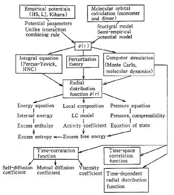
Figure 2.2.1. A scheme for the design of molecular ensembles.
sion of additivity rule, which has now an empirical character. It is however useful for practical purposes.
2.2.5 MODEL SYSTEM AND PARADIGM FOR DESIGN
The method described above is so to speak an orthodox approach and the ability of pres- ent-day’s supercomputer is still a high wall in the application of molecular simulation. Then the role of the second method given in the last section is highly expected.
It is the method with empirical potential model. As the model, the approximation that any molecule can behave as if obeying Lennard-Jones potential seems to be satisfactory. This (one-center) LJ model is valid only for rare gases and simple spherical molecules. But this model may also be valid for other simple molecules as a zeroth approximation. We may also use two-center LJ model where interatomic interactions are concentrated to the major two atoms in the molecule. We expect that these one-center and two-center LJ models will play a role of Occam’s razor.
We propose a paradigm for physical properties prediction as shown in Figure 2.2.1. This corresponds to the stage (2) and may be used to prepare the process of stage (3), namely, the molecular ensemble design for solvents.
Main procedures in this paradigm are as follows; we first adopt target molecule or mixture and determine their LJ parameters. At present stage, LJ parameters are available only for limited cases. Thus we must have method to predict effective LJ parameters.

2.2 Molecular design of solvents |
41 |
For any kinds of mixtures, in addition to LJ parameters for each component, combining rule (or mixing rule) for unlike interaction should be prepared. Even for simple liquid mixtures, conventional Lorentz-Berthelot rule is not good answer.
Once potential parameters have been determined, we can start calculation downward following arrow in the figure. The first key quantity is radial distribution function g(r) which can be calculated by the use of theoretical relation such as Percus-Yevick (PY) or Hypernetted chain (HNC) integral equation. However, these equations are an approximations. Exact values can be obtained by molecular simulation. If g(r) is obtained accurately as functions of temperature and pressure, then all the equilibrium properties of fluids and fluid mixtures can be calculated. Moreover, information on fluid structure is contained in g(r) itself.
On the other hand, we have, for non-equilibrium dynamic property, the time correlation function TCF, which is dynamic counterpart to g(r). One can define various TCF’s for each purpose. However, at the present stage, no extensive theoretical relation has been derived between TCF and φ(r). Therefore, direct determination of self-diffusion coefficient, viscosity coefficient by the molecular simulation gives significant contribution in dynamics studies.
Concluding Remarks
Of presently available methods for the prediction of solvent physical properties, the solubility parameter theory by Hildebrand10 may still supply one of the most accurate and comprehensive results. However, the solubility parameter used there has no purely molecular character. Many other methods are more or less of empirical character.
We expect that the 21th century could see more computational results on solvent properties.
REFERENCES
1N. Metropolis, A. W. Rosenbluth, M. N. Rosenbluth, A. H. Teller and E. Teller, J. Chem. Phys., 21, 1087 (1953).
2B. J. Alder and T. E. Wainwright, J. Chem. Phys., 27, 1208 (1957).
3(a) M. P. Allen and D. J. Tildesley, Computer Simulation of Liquids, Clarendon Press, Oxford, 1987.
(b)R. J. Sadus, Molecular Simulation of Fluids, Elsevier, Amsterdam, 1999.
4R. C. Reid, J. M. Prausnitz and J. E. Poling, The Properties of Gases and Liquids; Their Estimation and
Prediction, 4th Ed., McGraw-Hill, New York, 1987.
5C. R. Wilke and P. Chang, AIChE J., 1, 264 (1955).
6K. Nakanishi, Ind. Eng. Chem. Fundam., 17, 253 (1978).
7 O. Matsuoka, E. Clementi and M. Yoshimine, J. Chem. Phys., 60, 1351 (1976). 8 S. Okazaki, K. Nakanishi and H. Touhara, J. Chem. Phys., 78, 454 (1983).
9W. L. Jorgensen, J. Am. Chem. Soc., 103, 345 (1981).
10 J. H. Hildebrand and R. L. Scott, Solubility of Non-Electrolytes, 3rd Ed., Reinhold, New York, 1950.
APPENDIX
PREDICTIVE EQUATION FOR THE DIFFUSION COEFFICIENT IN DILUTE SOLUTION
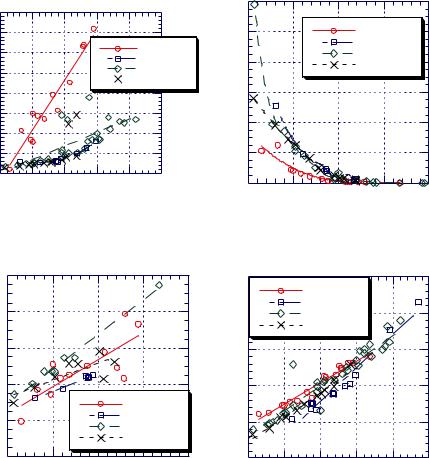
Experimental evidence is given in Figure 2.2.2 for the prediction based on equation [2.2.1]. The diffusion coefficient D0 of solute A in solvent B at an infinite dilution can be calculated using the following equation:
|
|
9.97 10−8 |
|
2.40 10−8 A |
S V |
|
T |
|
||
|
|
= |
|
|
|
B |
B B |
|
|
|
D |
0 |
|
|
+ |
|
|
|
|
[2.2.3] |
|
|
|
|
|
|
||||||
|
|
[I V |
]1/ 3 |
|
I A SAVA |
|
|
ηB |
|
|
|
|
|
|
|
||||||
|
|
|
A A |
|
|
|
|
|
|
|

42 |
Koichiro Nakanishi |
Figure 2.2.2. Hammond-Stokes plot for diffusion of iodine and carbon tetrachloride in various solvents at
298.15K. o, ,: D1η2, n: (D1)selfη2, •: D1η2 at the Stokes-Einstein limit. Perpendicular lines connect two or more data for the same solvent from different sources. [Adapted, by permission, from K. Nakanishi, Bull. Chem. Soc. Ja-
pan, 51, 713 (1978).
where D0 is in cm2 s-1. VA and VB are the liquid molar volumes in cm3 mol-1 of A and B at the temperature T in K, and the factors I, S, and A are given in original publications,4,6 and η is the solvent viscosity, in cP.
Should the pure solute not be a liquid at 298 K, it is recommended that the liquid volume at the boiling point be obtained either from data or from correlations.4 Values of D0 were estimated for many (149) solute-solvent systems and average error was 9.1 %.
2.3 BASIC PHYSICAL AND CHEMICAL PROPERTIES OF SOLVENTS
George Wypych
ChemTec Laboratories, Inc., Toronto, Canada
This section contains information on the basic relationships characterizing the physical and chemical properties of solvents and some suggestions regarding their use in solvent evaluation and selection. The methods of testing which allow us to determine some of physical and chemical properties are found in Chapter 15. The differences between solvents of various chemical origin are discussed in Chapter 3, Section 3.3. The fundamental relationships in this chapter and the discussion of different groups of solvents are based on extensive CD-ROM database of solvents which can be obtained from ChemTec Publishing. The database has 110 fields which contain various data on solvent properties which are discussed below. The database can be searched by the chemical name, empirical formula, molecular weight, CAS number and property. In the first case, full information on a particular solvent
2.3 Basic physical and chemical properties |
43 |
is returned. In the second case, a list of solvents and their values for the selected property are given in tabular form in ascending order of the property in question.
2.3.1 MOLECULAR WEIGHT AND MOLAR VOLUME
The molecular weight of a solvent is a standard but underutilized component of the information on properties of solvents. Many solvent properties depend directly on their molecular weights. The hypothesis of Hildebrand-Scratchard states that solvent-solute interaction occurs when solvent and polymer segment have similar molecular weights. This is related to the hole theory according to which a solvent occupying a certain volume leaves the same volume free when it is displaced. This free volume should be sufficient to fit the polymer segment which takes over the position formerly occupied by the solvent molecule.
Based on this same principle, the diffusion coefficient of a solvent depends on its molecular mass (see equations [6.2] and [6.3]). As the molecular weight of a solvent increases its diffusion rate also increases. If there were no interactions between solvent and solute, the evaporation rate of the solvent would depend on the molecular weight of the solvent. Because of various interactions, this relationship is more complicated but solvent molecular weight does play an essential role in solvent diffusion. This is illustrated best by membranes which have pores sizes which limit the size of molecules which may pass through. The resistance of a material to solvents will be partially controlled by the molecular weight of the solvent since solvent molecules have to migrate to the location of the interactive material in order to interact with it.
The chemical potential of a solvent also depends on its molecular weight (see eq. [6.6]). If all other influences and properties are equal, the solvent having the lower molecular weight is more efficiently dissolving materials, readily forms gels, and swells materials. All this is controlled by the molecular interactions between solvent and solute. In other words, at least one molecule of solvent involved must be available to interact with a particular segment of solute, gel, or network. If solvent molecular weight is low more molecules per unit weight are available to affect such changes. Molecular surface area and molecular volume are part of various theoretical estimations of solvent properties and they are in part
|
|
|
|
|
|
|
|
|
|
|
|
|
|
|
|
|
|
|
|
|
|
|
|
|
|
|
|
|
|
|
|
|
|
|
|
|
|
|
|
|
|
|
|
|
|
|
|
|
|
|
|
|
|
dependent on the molecular mass of the sol- |
-3 |
25 |
|
|
|
|
|
|
|
|
|
|
|
|
|
|
|
|
|
|
|
|
|
|
|
|
|
|
|
|
|
|
|
|
|
|
|
|
|
|
|
|
|
|
|
|
|
|
|
|
|
|
|
|
vent. |
cm |
|
|
|
|
|
|
|
|
|
|
|
|
|
|
|
|
|
|
|
|
|
|
|
|
|
|
|
|
|
|
|
|
|
|
|
|
|
|
|
|
|
|
|
|
|
|
|
|
|
|
|
|
||
, cal |
|
|
|
|
|
|
|
|
|
|
|
|
|
|
|
|
|
|
|
|
|
|
|
|
|
|
|
|
|
|
|
|
|
|
|
|
|
|
|
|
|
|
|
|
|
|
|
|
|
|
|
|
|
Many physical properties of solvents |
|
|
|
|
|
|
|
|
|
|
|
|
|
|
|
|
|
|
|
|
|
|
|
|
|
|
|
|
|
|
|
|
|
|
|
|
|
|
|
|
|
|
|
|
|
|
|
|
|
|
|
|
|
depend on their molecular weight, such as |
|
|
|
|
|
|
|
|
|
|
|
|
|
|
|
|
|
|
|
|
|
|
|
|
|
|
|
|
|
|
|
|
|
|
|
|
|
|
|
|
|
|
|
|
|
|
|
|
|
|
|
|
|
|
||
parameter,δ |
20 |
|
|
|
|
|
|
|
|
|
|
|
|
|
|
|
|
|
|
|
|
|
|
|
|
|
|
|
|
|
|
|
|
|
|
|
|
|
|
|
|
|
|
|
|
|
|
|
|
|
|
|
|
boiling and freezing points, density, heat of |
|
|
|
|
|
|
|
|
|
|
|
|
|
|
|
|
|
|
|
|
|
|
|
|
|
|
|
|
|
|
|
|
|
|
|
|
|
|
|
|
|
|
|
|
|
|
|
|
|
|
|
|
|||
|
|
|
|
|
|
|
|
|
|
|
|
|
|
|
|
|
|
|
|
|
|
|
|
|
|
|
|
|
|
|
|
|
|
|
|
|
|
|
|
|
|
|
|
|
|
|
|
|
|
|
|
|
evaporation, flash point, and viscosity. The |
|
|
|
|
|
|
|
|
|
|
|
|
|
|
|
|
|
|
|
|
|
|
|
|
|
|
|
|
|
|
|
|
|
|
|
|
|
|
|
|
|
|
|
|
|
|
|
|
|
|
|
|
|
|
||
15 |
|
|
|
|
|
|
|
|
|
|
|
|
|
|
|
|
|
|
|
|
|
|
|
|
|
|
|
|
|
|
|
|
|
|
|
|
|
|
|
|
|
|
|
|
|
|
|
|
|
|
|
|
relationship between these properties and |
|
|
|
|
|
|
|
|
|
|
|
|
|
|
|
|
|
|
|
|
|
|
|
|
|
|
|
|
|
|
|
|
|
|
|
|
|
|
|
|
|
|
|
|
|
|
|
|
|
|
|
|
|
|||
|
|
|
|
|
|
|
|
|
|
|
|
|
|
|
|
|
|
|
|
|
|
|
|
|
|
|
|
|
|
|
|
|
|
|
|
|
|
|
|
|
|
|
|
|
|
|
|
|
|
|
|
molecular weight for a large number of sol- |
||
|
|
|
|
|
|
|
|
|
|
|
|
|
|
|
|
|
|
|
|
|
|
|
|
|
|
|
|
|
|
|
|
|
|
|
|
|
|
|
|
|
|
|
|
|
|
|
|
|
|
|
|
|||
solubility |
|
|
|
|
|
|
|
|
|
|
|
|
|
|
|
|
|
|
|
|
|
|
|
|
|
|
|
|
|
|
|
|
|
|
|
|
|
|
|
|
|
|
|
|
|
|
|
|
|
|
|
|
|
vents of different chemical composition is |
|
|
|
|
|
|
|
|
|
|
|
|
|
|
|
|
|
|
|
|
|
|
|
|
|
|
|
|
|
|
|
|
|
|
|
|
|
|
|
|
|
|
|
|
|
|
|
|
|
|
|
|
|
||
10 |
|
|
|
|
|
|
|
|
|
|
|
|
|
|
|
|
|
|
|
|
|
|
|
|
|
|
|
|
|
|
|
|
|
|
|
|
|
|
|
|
|
|
|
|
|
|
|
|
|
|
|
|
affected by numerous other influences but |
|
|
|
|
|
|
|
|
|
|
|
|
|
|
|
|
|
|
|
|
|
|
|
|
|
|
|
|
|
|
|
|
|
|
|
|
|
|
|
|
|
|
|
|
|
|
|
|
|
|
|
|
|
|||
|
|
|
|
|
|
|
|
|
|
|
|
|
|
|
|
|
|
|
|
|
|
|
|
|
|
|
|
|
|
|
|
|
|
|
|
|
|
|
|
|
|
|
|
|
|
|
|
|
|
|
|
|||
|
|
|
|
|
|
|
|
|
|
|
|
|
|
|
|
|
|
|
|
|
|
|
|
|
|
|
|
|
|
|
|
|
|
|
|
|
|
|
|
|
|
|
|
|
|
|
|
|
|
|
|
within the same chemical group (or similar |
||
|
|
|
|
|
|
|
|
|
|
|
|
|
|
|
|
|
|
|
|
|
|
|
|
|
|
|
|
|
|
|
|
|
|
|
|
|
|
|
|
|
|
|
|
|
|
|
|
|
|
|
|
|||
|
|
|
|
|
|
|
|
|
|
|
|
|
|
|
|
|
|
|
|
|
|
|
|
|
|
|
|
|
|
|
|
|
|
|
|
|
|
|
|
|
|
|
|
|
|
|
|
|
|
|
|
|
||
Hildebrand |
|
|
|
|
|
|
|
|
|
|
|
|
|
|
|
|
|
|
|
|
|
|
|
|
|
|
|
|
|
|
|
|
|
|
|
|
|
|
|
|
|
|
|
|
|
|
|
|
|
|
|
|
|
structure) molecular weight of solvent cor- |
|
|
|
|
|
|
|
|
|
|
|
|
|
|
|
|
|
|
|
|
|
|
|
|
|
|
|
|
|
|
|
|
|
|
|
|
|
|
|
|
|
|
|
|
|
|
|
|
|
|
|
|
|
||
5 |
|
|
|
|
|
|
|
|
|
|
|
|
|
|
|
|
|
|
|
|
|
|
|
|
|
|
|
|
|
|
|
|
|
|
|
|
|
|
|
|
|
|
|
|
|
|
|
|
|
|
|
|
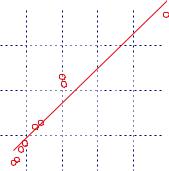
relates well with its physical properties. |
|
0 |
|
|
500 1000 1500 2000 2500 |
Figure 2.3.1 gives an example of in- |
||||||||||||||||||||||||||||||||||||||||||||||||||
|
|
|
|
-1 |
|
|
|
|
|
|
|
|
terrelation of seemingly unrelated parame- |
|||||||||||||||||||||||||||||||||||||||||
|
|
|
|
|
|
|
|
|
|
|
|
|
||||||||||||||||||||||||||||||||||||||||||
|
|
|
|
|
|
|
Heat of vaporization, kJ kg |
|
||||||||||||||||||||||||||||||||||||||||||||||
|
|
|
|
|
|
|
|
|
|
|
|
|
|
|
|
|
|
|
|
|
|
|
|
|
|
|
|
|
|
|
|
|
|
|
|
|
|
|
|
|
|
|
|
|
|
|
|
|
|
|
|
|
|
ters: Hildebrand solubility parameter and |
Figure 2.3.1. Hildebrand solubility parameter vs. heat of |
heat of vaporization (see more on the sub- |
|||||||||||||||||||||||||||||||||||||||||||||||||||||
vaporization of selected solvents. |
|
|||||||||||||||||||||||||||||||||||||||||||||||||||||

44 |
George Wypych |
ject in the Section 2.3.19). As heat of vaporization increases, the solubility parameter also increases.
Molar volume is a rather speculative, theoretical term. It can be calculated from Avogadro’s number but it is temperature dependent. In addition, free volume is not taken into consideration. Molar volume can be expressed as molecular diameter but solvent molecules are rather non-spherical therefore diameter is often misrepresentation of the real dimension. It can be measured from the studies on interaction but results differ widely depending on the model used to interpret results.
2.3.2 BOILING AND FREEZING POINTS
Boiling and freezing points are two basic properties of solvents often included in specifications. Based on their boiling points, solvents can be divided to low (below 100oC), medium (100-150oC) and high boiling solvents (above 150oC).
The boiling point of liquid is frequently used to estimate the purity of the liquid. A similar approach is taken for solvents. Impurities cause the boiling point of solvents to increase but this increase is very small (in the order of 0.01oC per 0.01% impurity). Considering that the error of boiling point can be large, contaminated solvents may be undetected by boiling point measurement. If purity is important it should be evaluated by some other, more sensitive methods. The difference between boiling point and vapor condensation temperature is usually more sensitive to admixtures. If this difference is more than 0.1oC, the presence of admixtures can be suspected.
The boiling point can also be used to evaluate interactions due to the association among molecules of solvents. For solvents with low association, Trouton’s rule, given by the following equation, is fulfilled:
Sbpo = |
Hbpo |
= 88J mol −1 K −1 |
[2.3.1] |
|
Tbp |
||||
|
|
|
||
where: |
|
|
|
|
So |
molar change of enthalpy |
|
||
bp |
|
|
|
|
Hbpo |
molar change of entropy |
|
||
Tbp |
boiling point |
|
||
If the enthalpy change is high it suggests that the solvent has a strong tendency to form associations.
Boiling point depends on molecular weight but also on structure. It is generally lower for branched and cyclic solvents. Boiling and freezing points are important considerations for solvent storage. Solvents are frequently stored under nitrogen blanket and they contribute to substantial emissions during storage. Freezing point of some solvents is above temperatures encountered in temperate climatic conditions. Although, solvents are usually very stable in their undercooled state, they rapidly crystallize when subjected to any mechanical or sonar impact.
Figures 2.3.2 to 2.3.6 illustrate how the boiling points of individual solvents in a group are related to other properties. Figure 2.3.2 shows that chemical structure of a solvent affects the relationship between its viscosity and the boiling point. Alcohols, in particular, show a much larger change in viscosity relative to boiling point than do aromatic hydrocarbons, esters and ketones. This is caused by strong associations between molecules of alcohols, which contain hydroxyl groups. Figure 2.3.3 shows that alcohols are also less volatile