Wypych Handbook of Solvents

Both the hydrophobicity and hydrogen bonding property of the solutes seem to be important in influencing the extent of the deviation from the ideal log-linear pattern.

Additional deviations related to the solute’s behavior may occur. For organic electrolytes, the acid dissociation constant Ka may decrease as cosolvent fraction f increases.40,75,92 This, in turn, will affect the patterns of solubilization by cosolvents. Furthermore, a high concentration of solutes may invalidate the log-linear model, which presumes negligible volume fraction of solute and no solute-solute interactions. For solid solutes, solvent induced polymorphism may also bring additional changes in their solubilization profile.

Another approach to quantitatively address the deviations of solubilization from the log-linear model makes use of an empirical parameter β:

The modified log-linear equation then takes the form:

Under the assumptions that the solute is chemically stable and has little influence on the activity of solvent component, β reflects the extent of deviation caused by the nonideality of the solvent mixture, as suggested by Rao et al.28 However, since β itself is a complicated function of f, equation [14.21.2.13] does not provide additional aid for predicting cosolvency.

14.21.2.7 Summary

Applications of cosolvency in pharmaceutical and environmental research and industries are briefly summarized. Using ethanol as an example, the effects of adding a cosolvent on the solubilities of various organic solutes are presented in Figure 14.21.2.1. The log-linear solubilization model, equation [14.21.2.2] or [14.21.2.4], is the simplest theory of cosolvency developed so far. It discovers general trends and major determinant factors of cosolvency, thus providing guidelines for predicting solubility of organic chemicals in mixed solvents. The cosolvency power of a specific cosolvent towards a solute of interest, σ, can be estimated with equation [14.21.2.5] with the knowledge of the solute octanol-wa- ter partition coefficient Kow. Sources of error associated with this estimation method are discussed based on equation [14.21.2.6]. The slope of the σ~log Kow regression, b, can be

estimated from the log Kow and hydrogen bond donor density of the cosolvent, as presented by equation [14.21.2.8]. One of the previously published modifications to the log-linear model, equation [14.21.2.10], is evaluated. The difference between the measured log Sm and those predicted by the log-linear and the extended log-linear model are presented in Figure 14.21.2.2 for solutes naphthalene, benzocaine, and benzoic acids in selected water and cosolvent mixtures.

Notations

aintercept of σ ~ log Kow regression

bslope of σ ~ log Kow regression

fvolume fraction of cosolvent in mixed solvent with water.

βempirically obtained water-cosolvent interaction parameter

σcosolvency power, σ = log (Sc/Sw)

References

1 A. Martin, J. Newburger, and A. Adjel, J. Pharm. Sci., 68, 4 (1979).

2 A. Martin, J. Newburger, and A. Adjel, J. Pharm. Sci., 69, 487 (1980).

3A. Martin, A. N. Paruta, and A. Adjel, J. Pharm. Sci., 70, 1115 (1981).

4 P. Bustamante, B. Escalera, A. Martin, and E. Selles, Pharm. Pharmacol., 45, 253 (1993). 5 N. A. Williams, and G. L. Amidon, J. Pharm. Sci., 73, 9 (1984).

6 N. A. Williams, and G. L. Amidon, J. Pharm. Sci., 73, 14 (1984).

7 N. A. Williams, and G. L. Amidon, J. Pharm. Sci., 73, 18 (1984).

8 D. Khossrani, and K. A. Connors, J. Pharm. Sci., 82, 817 (1993).

9D. Khossravi, and K. A. Connors, J. Pharm. Sci., 81, 371 (1992).

10A. Jouyban-Gharamaleki, Chem. Pharm. Bull., 46, 1058 (1998).

11W. E. Acree, Jr., J. W. McCargar, A. I. Zvaigzne, and I. L. Teng, Phys. Chem. Liq., 23, 27 (1991)

12W. E. Acree, Jr. and A. I. Zvaigzne, Thermochimica. Acta, 178, 151 (1991).

13A. B. Ochsner, R. J. Belloto Jr., and T. D. Sololoski, J. Pharm. Sci., 74, 132 (1985).

14M. Barzegar-Jalali, and J. Hanaee, Int. J. Pharm., 109, 291 (1994).

15A. Li, and A. W. Andren, Environ. Sci. Technol., 29, 3001 (1995).

16J. K. Fu, and R. G. Luthy, J. Environ. Eng., 112, 328 (1986).

17M. Barzegar-Jalali, and A. Jouyban-Gharamaleki, Int. J. Pharm., 140, 237 (1996).

18R. M. Dickhut, D. E. Armstrong, and A. W. Andren, Environ. Toxicol. Chem., 10, 881 (1991).

19A. Jouyban-Gharamaleki, L. Valaee, M. Barzegar-Jalali, B. J. Clark, and W. E. Acree, Jr., Intern. J. Pharm., 177, 93 (1999).

20S. H. Yalkowsky, in Techniques of solubilization of drugs; S. H. Yalkowsky, Ed.; Dekker, New York, 1984, Chapter 1.

21S. C. Smolinske, Handbook of Food, Drug, and Cosmetic Excipients, CRC Press, Ann Arbor, MI, 1992.

22F. Herzel, and A. S. Murty, Bull. Environ. Toxicol., 32, 53 (1984).

23C. Munz, and P. Roberts, Environ. Sci. Technol., 20, 830 (1986).

24K. R. Morris, R. Abramowitz, R. Pinal, P. Davis, and S. H. Yalkowsky, Chemosphere, 17, 285 (1988).

25F. R. Groves, Jr, Environ. Sci. Technol., 22, 282 (1988).

26R. M. Dickhut, A. W. Andren, and D. E. Armstrong, J. Chem. Eng. Data, 34, 438 (1989).

27R. Pinal, P. S. C. Rao, L. S. Lee, P. V. Cline, and S. H. Yalkowsky, Environ. Sci. Technol., 24, 639 (1990).

28P. S. C. Rao, L. S. Lee, and A. L. Wood, EPA/600/M-91/009 (1991).

29A. Li, W. J. Doucette, and A. W. Andren, Chemosphere, 24, 1347 (1992).

30A. Li, and A. W. Andren, Environ. Sci. Technol., 28, 47 (1994).

31A. Li, A. W. Andren, and S. H. Yalkowsky, Environ. Toxicol. Chem., 15, 2233 (1996).

32P. Nkedi-Kizza, P. S. C. Rao, and A. G. Hornsby, Environ. Sci. Technol., 19, 975 (1985).

33J. K. Fu, and R. G. Luthy, J. Environ. Eng., 112, 346 (1986).

34R. W. Walters, and A. Guiseppl-Elie, Environ. Sci. Technol., 22, 819 (1988).

35P. Nkedi-Kizza, M. L. Brusseau, P. S. C. Rao, and A. G. Hornsby, Environ. Sci. Technol., 23, 814 (1989).

36A. L. Wood, D. C. Bouchard, M. L. Brusseau, and P. S. C. Rao, Chemosphere, 21, 575 (1990).

37P. S. C. Rao, L. S. Lee, and R. Pinal, Environ. Sci. Technol., 24, 647 (1990).

38F. C. Spurlock, and J. W. Biggar, Environ. Sci. Technol., 28, 1003 (1994).

39W. J. M. Hegeman, C. H. Van der Weijden, and J. P. G. Loch, Environ. Sci. Technol., 29, 363 (1995).

40L. S. Lee, and P. S. C. Rao, Environ. Sci. Technol., 30, 1533 (1996).

41V. A. Nzengung, E. A. Voudrias, P. Nkedi-Kizza, J. M. Wampler, and C. E. Weaver, Environ. Sci. Technol., 30, 89 (1996).

42R. P. Singh, Colloids and Surfaces A., 122, 63 (1997).

43V. A. Nzengung, P. Nkedi-Kizza, R. E. Jessup, and E. A. Voudrias, Environ. Sci. Technol., 31, 1470 (1997).

44T. C. Harmon, T. J. Kim, B. K. D. Barre, and C. V. Chrysikopoulos, J. Environ. Eng., January, 87 (1999).

45M. A. Ei-Zoobi, G. E. Ruch, and F. R. Groves Jr., Environ. Sci. Technol., 24, 1332 (1990).

46W. F. Lane, and R. C. Loehr, Environ. Sci. Technol., 26, 983 (1992).

47C. S. Chen, and J. J. Delfino, J. Environ. Eng., April 354 (1997).

48G. R. Jones, Environ. Prog., 11, 223 (1992).

49USEPA, Assessment and Remediation of contaminated Sediments (ARCS) Program: Remediation Guidance Document. EPA 905-R94-003, (1994) p.180.

50USEPA, EPA 542-K-94-006 (1995).

51C. T. Jafvert, Ground-Water Remediation Technologies Analysis Center, Echnology Evaluation Report, TE-96-02 (1996).

52R. W. Falta, GWMR, Summer, 94 (1998).

53D. C. M. Augustijin, R. E. Jessup, P. S. Rao, and A. L. Wood, J. Environ. Eng., 120, 42 (1994).

54R. K. Sillan, M. D. Annable, P. S. C. Rao, D. Dai, K. Hatfield, W. D. Graham, A. L. Wood, and C. G. Enfield,

Water Resources Res., 34, 2191 (1998).

55P. S. C. Rao, M. D. Annable, R. K. Sillan, D. Dai, K. Hatfield, and W. D. Graham, Water Resources Res., 33, 2673 (1997).

56J. W. Jawitz, M. D. Annable, P. S. C. Rao, and R. D. Rhue, Environ. Sci. Technol., 32, 523 (1998).

57A. T. Kan, M. B. Tomson, and T. A. McRae, Proceedings of the 203rd American Chemical Society National Meeting, San Francisco, CA (1992).

58D. Brandes, and K. J. Farley, J. Water Environ. Res., 65, 869 (1993).

59A. Li, K. A. Cheung, and K. Reddy, J. Environ. Eng., 126, 527 (2000).

60A. Li, and S. H. Yalksowsky, J. Pharm. Sci., 83, 1735 (1994).

61S. H. Yalkowsky, and T. J. Roseman, in Techniques of solubilization of drugs; S. H. Yalkowsky, Ed.; Dekker, New York, 1984, Chapter 3.

62J. T. Rubino, and S. H. Yalkowsky, J. Pharm. Sci., 74, 416 (1985).

63P. J. Leinonen, and D. Mackay, Can. J. Chem. Eng., 51, 230 (1973).

64R. P. Eganhouse, and J. A. Calder, Geochimca et Cosmochimica Acta, 40, 555 (1976).

65Y. B. Tewari, D. E. Martire, S. P.; Wasik, and M. M. Miller, J. Solution Chem., 11, 435 (1982).

66S. Banerjee, Environ. Sci. Technol., 18, 587 (1984).

67D. R. Burris, and W. G. MacIntyre, Environ. Toxicol. Chem., 4, 371 (1985).

68H. H. Hooper, S. Michel, and J. M. Prausnitz, J. Chem. Eng. Data, 33, 502 (1988).

69D. Mackay, J. Contam. Hydrol. 8, 23 (1991).

70A. Li, and W. J. Doucette, Environ. Toxicol. Chem., 12, 2031 (1993).

71S. Lesage, and S. Brown, J. Contam. Hydrol., 15, 57 (1994).

72K. Brololm, and S. Feenstra, Environ. Toxicol. Chem., 14, 9 (1995).

73G. T. Coyle, T. C. Harmon, and I. H. Suffet, Environ. Sci. Technol., 31, 384 (1997).

74P. S. C. Rao, L. S. Lee, P. Nkedi-Kizza, and S. H. Yalkowsky, in Toxic Organic Chemicals in Porous Media, Z. Gerstl, Eds. Springer-Verlag, New York, 1989, Chapter 8.

75R. Pinal, L. S. Lee, and P. S. C. Rao, Chemosphere, 22, 939 (1991).

76S. H. Yalkowsky, and J. T. Rubino, J. Pharm. Sci., 74, 416 (1985).

77J. T. Rubino, and S. H. Yalkowsky, J. Parent. Sci. Technol., 41, 172 (1984).

78W. J. Lyman, W. f. Reehl, and D. H. Rosenblatt, Handbook of Chemical Property Estimation Methods: Environmental Behavior of Organic Compounds. ACS Publications, Washington, DC, 1990.

79C. Hansch, and A. J. Leo, Substituent constants for Correlation Analysis in Chemistry and Biology.

John Wiley, New York, 1979.

80A. Li, and S. H. Yalkowsky, Ind. Eng. Chem. Res., 37, 4470 (1998).

81J. T. Rubino, and S. H. Yalkowsky, Pharm. Res., 4, 220 (1987).

82A. Li, and S. H. Yalkowsky, Ind. Eng. Chem. Res., 37, 4476 (1998).

83R. Abramowitz, Ph.D. Dissertation, University of Arizona, 1986.

84A. Li, and S. H. Yalkowsky, unpublished data.

85J. T. Rubino, Ph.D. Dissertation, University of Arizona, 1984.

86S. H. Yalkowsky, unpublished data.

87J. T. Rubino, and S. H. Yalkowsky, Pharm. Res., 4, 231 (1987).

88A. Fredenslund, R. L. Jones, and J. M. Prausnitz, A.I.Ch.E. J., 21, 1086 (1975).

89J. Gmehling, P. Rasmussen, and A. Fredenslund, Ind. Eng. Chem. Process Des. Dev., 21, 118 (1982).

90E. A. Macedo, U. Weidlich, J. Gmehling, and P. Rasmussen, Ind. Eng. Chem. Process Des. Dev., 22, 678 (1983).

91J. T. Rubino, and E. K. Obeng, J. Pharm. Sci., 80, 479 (1991).

92L. S. Lee, C. A. Bellin, R. Pinal, and P. S. C. Rao, Environ. Sci. Technol., 27, 165 (1997).

14.22 POLYMERS AND MAN-MADE FIBERS

George Wypych

ChemTec Laboratories, Inc., Toronto, Canada

The resin production industry has over 450 plants in the USA with total sales of $33 billion/year and about 60,000 employees. The man-made fiber industry has over 90 plants. It employs about 45,000 people and it has sales of $13 billion/year.

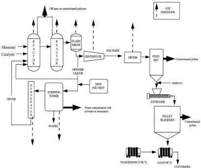
In the polymer manufacture industry, production processes are diverse both in technology and equipment design. They have common steps which include preparation of reactants, polymerization, polymer recovery, polymer extrusion (if in pelletized form), and supporting operations. In some preparation operations, solvents are used to dissolve or dilute monomer and reactants. Solvent are also used to facilitate the transportation of the reaction mixture throughout the plant, to improve heat dissipation during the reaction, and to promote uniform mixing. Solvent selection is optimized to increase monomer ratio and to reduce polymerization costs and emissions. The final polymer may or may not be soluble in the solvent. These combinations of polymers and solvents are commonly used: HDPE - isobutane and hexane, LDPE - hydrocarbons, LLDPE - octene, butene, or hexene, polypropylene - hexane, heptane or liquid propylene, polystyrene - styrene or ethylbenzene, acrylic - dimethylacetamide or aqueous inorganic salt solutions. These examples show that there are options available. Excess monomer may replace solvent or water can be used as the solvent. During polymer recovery unreacted monomer and solvents are separated from polymer (monomers and solvents are flashed off by lowering the pressure and sometimes degassing under vacuum), liquids and solids are separated (the polymer may be washed to remove sol-

Figure 14.22.1. Schematic diagram of emissions from the polymer manufacturing industry. [Reproduced from EPA Office of Compliance Sector Notebook Project. Profile of the Petroleum Refining Industry. US Environmental Protection Agency, 1995.]

vent), and residual water and solvent are purged during polymer drying. Residual solvents are removed by further drying and extrusion. Solvents are also used in equipment cleaning. Solvents are often stored under a nitrogen blanket to minimize oxidation and contamination. When these systems are vented solvent losses occur. Figure 14.22.1 shows a schematic diagram of potential emissions during polymer manufacture.

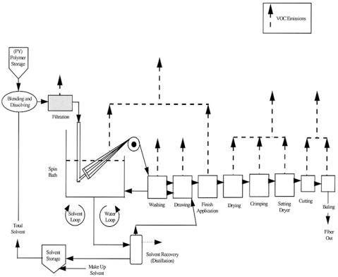
Manufacture of man-made fibers involves polymerization (usually the core part of the process), preparation of the solution, spinning, washing and coagulation, drying and other operations. Fibers are formed by forcing the viscous liquid through small-bore orifices. A suitable viscosity can be achieved either by heating or dissolution. The rheological properties of the solution are governed to a large degree by the solvents selected. Wastes generated during the spinning operation include evaporated solvent and wastewater contaminated by solvent. The typical solvents used in the production of fibers are dimethylacetamide (acrylic), acetone or chlorinated hydrocarbon (cellulose acetate), and carbon disulfide (rayon). In the dry spinning process a solution of polymer is first prepared. The solution is then heated above the boiling temperature of the solvent and the solution is extruded through spinneret. The solvent evaporates into the gas stream. With wet spinning the fiber is directly extruded into a coagulation bath where solvent diffuses into the bath liquid and the coagulant diffuses into the fiber. The fiber is washed free of solvent by passing it through an additional bath. Each process step generates emissions or wastewater. Solvents used in production are normally recovered by distillation. Figure 14.22.2 is a schematic diagram of fiber production showing that almost all stages of production generate emissions.

Figure 14.22.2. Schematic diagram of emissions from the man-made fiber manufacturing industry. [Reproduced from EPA Office of Compliance Sector Notebook Project. Profile of the Petroleum Refining Industry. US Environmental Protection Agency, 1995.]

Tables 14.22.1 and 14.22.2 provide data on releases and transfers from both polymer manufacturing and man-made fiber production in the USA. Carbon disulfide, methanol, xylene, and ethylene glycol are used in the largest quantities. Carbon disulfide is used in manufacture of regenerated cellulose and rayon. Ethylene glycol is used in the manufacture of polyethylene terephthalate, the manufacture of alkyd resins, and as cosolvent for cellulose ethers and esters. Methanol is used in several processes, the largest being in the production of polyester. This industry is the 10th largest contributor of VOC and 7th largest in releases and transfers.

There have been many initiatives to reduce emissions and usage of solvents. Man-made fiber manufacturing no longer uses benzene. DuPont eliminated o-xylene and reduced methanol and ethylene glycol use in its Wilmington operation. This change resulted in annual savings of $1 million. Process modification in a polymer processing plant resulted in a decrease in total emissions of 74% and a reduction in the release of cyclohexane by 96%. Monitoring of thousands of valves in Eastman Texas plant resulted in a program of valve replacement which eliminated 99% of the emissions. Plant in Florida eliminated solvents from cleaning and degreasing. These examples show that in many cases pollution can be reduced by better equipment, organization, and care.

Table 14.22.1 Reported solvent releases from the polymer and man-made fiber industry in 1995 [Data from Ref. 1]

Table 14.22.2. Reported solvent transfers from the polymer and man-made fiber industry in 1995 [Data from Ref. 1]

New technology is emerging to reduce solvent use. Recent inventions disclose that, in addition to reducing solvents, the stability of ethylene polymers can be improved with the new developed process.3 A proper selection of solvent improved a stripping operation and contributed to the better quality of cyclic esters used as monomers.4 Solvent was used for the recovery of fine particles of polymer which were contaminating water.5 A new process for producing fiber for cigarette filters uses reduced amounts of solvent.6 Optical fibers are manufactured by radiation curing which eliminates solvents.7 A new electrospinning process has been developed which produces unique fibers by the dry spinning method, providing a simpler separation and regeneration of the solvent.8

REFERENCES

1EPA Office of Compliance Sector Notebook Project. Profile of the Petroleum Refining Industry.

US Environmental Protection Agency, 1995.

2EPA Office of Compliance Sector Notebook Project. Sector Notebook Data Refresh - 1997. US Environmental Protection Agency, 1998.

3M M Hughes, M E Rowland. C A Strait, US Patent 5,756,659, The Dow Chemical Company, 1998.

4D W Verser, A Cheung, T J Eggeman, W A Evanko, K H Schilling, M Meiser, A E Allen, M E Hillman, G E Cremeans, E S Lipinsky, US Patent 5,750,732, Chronopol, Inc., 1998.

5 H Dallmeyer, US Patent 5,407,974, Polysar Rubber Corporation, 1995. 6 J N Cannon, US Patent 5,512,230, Eastman Chemical Company, 1996.

7P J Shustack, US Patent 5,527,835, Borden, Inc., 1996.

8A E Zachariades, R S Porter, J Doshi, G Srinivasan, D H Reneker, Polym. News, 20, No.7, 206-7 (1995).

14.23PRINTING INDUSTRY

George Wypych

ChemTec Laboratories, Inc., Toronto, Canada

The number of printing and publishing operations in the US is estimated at over 100,000. 1.5 million people are employed. The value of shipments is over $135 billion. 97% of printing is done by lithography, gravure, flexography, letterpress, and screen printing on substrates such as paper, plastic metal, and ceramic. Although, these processes differ, the common feature is the use of cleaning solvents in imaging, platemaking, printing, and finishing operation. Most inks contain solvents and many of the adhesives used in finishing operations also contain solvents. Many processes use the so-called fountain solutions which are applied to enable the non-image area of the printing plate to repel ink. These solutions contain primarily isopropyl alcohol. But the printing operation is, by itself, the largest contributor of VOCs. Each printing process requires inks which differ drastically in rheology. For example, gravure printing requires low viscosity inks which contain a higher solvent concentrations.

Tables 14.23.1 and 14.23.2 provide data on the reported releases and transfers of solvents by the US printing industry. These data show that there are fewer solvents and relatively low releases and transfers compared with other industries. In terms of VOC contribution, the printing industry is 5th and 10th in the total emissions and transfers.

Current literature shows that there is extensive activity within and outside industry to limit VOCs and reduce emissions. Cleaning operations are the major influence on emissions. Shell has developed a new cleaning formulations containing no aromatic or chlori-