Wypych Handbook of Solvents

or saturated zone upgradient of the contaminated area. The solvent with the removed contaminants is then extracted downgradient and treated above ground. Precise formulations for the water/cosolvent mixture need to be determined by laboratory and pilot studies in order to achieve the desired removal.50-53

A few field-scale evaluations of this technique were carried out at Hill Air Force Base, Utah, where the aquifer had been severely contaminated by jet fuel, chlorinated solvents, and pesticides during 1940s and 1950s. These contaminants had formed a complex non-aqueous phase liquid (NAPL) containing more than 200 constituents, which covered the surfaces of soil particles and was trapped in pores and capillaries over the years. One of the evaluations consisted of pumping ternary cosolvent mixture (70% ethanol, 12% n-pen- tanol, and 18% water) through a hydraulically isolated test cell over a period of 10 days, followed by flushing with water for another 20 days.54,55 The removal efficiency varied from 90-99% at the top zone to 70-80% at the bottom near a confining clay layer. Similar removal efficiencies were obtained from another test cell using a combination of cosolvent n-penta- nol and a surfactant at a total of 5.5 wt % of the flushing solution.56 In order to remove gasoline residuals at a US Coast Guard base in Traverse City, Michigan, it was demonstrated that the contaminants were mobilized when cosolvent 2-propanol was used at 50% concentration, while methanol at either 20% or 50% showed little effect.57 Cosolvent flushing was also proven to be effective in treating NAPLs which were denser than water. Methanol, isopropanol, and t-butanol were used in treating soils contaminated with triand tetra-chlo- rinated ethylenes.58

The applicability of solvent flushing, however, is often limited by the characteristics of the soil, especially the particle size distribution. While sandy soils may result in uncontrolled fluid migration, clayey soils with particles size less than 60 m are often considered unsuitable for in situ solvent flushing due to low soil permeability. In an attempt to remove PAHs from poorly permeable soils, Li, et al.59 investigated the possibility of combining cosolvent flushing with the electrokinetic technique. Electrokinetic remediation involves application of a low direct electrical current to electrodes that are inserted into the ground. As water is continuously replenished at anodes, dissolved contaminants are flushed toward the cathode due to electroosmosis, where they can be extracted and further treated by various conventional wastewater treatment methods. Their column experiment of removing phenanthrene from soil was moderately successful with the assistance of cosolvent n-butylamine at 20%(v). Retardation factor (ratio of the water linear velocity to that of the chemical) of phenanthrene was reduced from 753 in pure water to 11 by the presence of n-butylamine, and 43% of the phenanthrene was removed after 127 days or 9 pore volumes. However, significant removal of phenanthrene was not attained in their experiments with acetone and hydrofuran as cosolvents.

14.21.2.4 Experimental observations

Numerous experimental data exist in the literature on the solubility of organic solutes, including both drugs and environmental pollutants, in various mixtures of water and cosolvents. Experimental observations are often illustrated by plotting the logarithm of solubility of the solute versus the volume fraction of cosolvent in the solvent mixture. A few examples of solubilization curves are shown in Figure 14.21.2.1, which shows three typical situations for solutes of different hydrophobicity in the mixture of water and ethanol.

The classification of solute/cosolvent/water systems based on their relative polarity was suggested by Yalkowsky and Roseman.61 Solutes which are less polar than both water

Figure 14.21.2.1. Effects of ethanol on the solubilities of selected organic compounds. (a): νbenzene, οnaphthalene, ¡ biphenyl, ↓anthracene, πbenzo(a)pyrene, ρperylene, ϒchrysene; (b) νhydantoic acid, οhydantoin, ϒ methyl hydantoic acic, ↓5-ethyl hydantoin, ρ5-isobutyl hydantoin; (c) οtriglycine, ϒdiglycine, ρglycine [Adapted, by permission, from Li and Yalkovsky, J. Pharm. Sci., 83, 1735 (1994).]

and the cosolvent are considered as “nonpolar”, those which have a polarity between those of water and the cosolvent as “semipolar”, and those which are more polar than both water and cosolvent as “polar”. Figure 14.21.2.1-a illustrates the behavior of relatively hydrophobic compounds, which tend to have monatonically increasing solubilization curves. The solubility enhancement is greater for the more hydrophobic solutes. Curves with opposite trends were mostly observed for polar solutes. The monatonical desolubilization is greater for more hydrophilic solutes, as evidenced by the curves in Figure 14.21.2.1-c. In-between are semipolar solutes with slightly parabolic curves shown in 14.21.2.1-b. The impact of adding cosolvents is much less profound for the semipolars than for the other two groups. On a linear solubility scale, the parabola tends to be more obvious than on the log scale. The same general trends were seen for the cosolvents glycerine61 and propylene glycol61,62 and presumably many other water-miscible cosolvents.

It is more difficult to evaluate the effects of cosolvents which have limited miscibility with water. In the literature, such organic solvents have been termed as both cosolvents and cosolutes, and there is no clear criteria for the distinction. Cosolvent is usually miscible with water, or to be used in an attempt to increase the aqueous solubility of the solute. Cosolute, on the other hand, may be organic chemicals which have a similar chemical structure or behave similarly with the solute when they exist in water alone. The effects of cosolutes have been examined in a limited number of published papers.63-73

Partially water-miscible organic solvents (PMOSs) may act as either cosolvents or cosolutes, and the research in the past has shown the complexity of their effects.23,27-30,73-75 It was demonstrated that in order to exert effects on solubility or sorption of HOCs, PMOSs must exist as a component of the solvent mixture in an appreciable amount: Munz and Roberts23 suggested a mole fraction of greater than 0.005 and Rao and coworkers27,28 proposed a volume percent of 1% or a concentration above 104 mg/L. Cosolvents with relatively high water solubility are likely to demonstrate observable effects on the solubilities of solutes, up to their solubility limits, in a similar manner to cosolvents of complete miscibility with water. A few experimental examples of the effects of PMOSs include 1-butanol and

1-pentanol acting on PCB congeners30 and naphthalene.26 and butanone on anthracene and fluoranthene.75

Even more hydrophobic organic solvents produce little or even negative influence on the solubility of HOCs. For instance, the presence of benzene does not increase the aqueous solubility of PCBs up to their saturation concentration.29 Solubility of a few PCB congeners in water were found to be depressed by dissolved dichloromethane and chloroform.73 On the other hand, PCB solubility showed little change when cosolvent benzyl alcohol, 1-hexanol, 1-heptanol, or 1-octanol was present.29,30 Similar “no change” observations were made for naphthalene with cosolvents dichloromethane and chloroform,73 and for solutes benzene and hexane with cosolvent MTBE.25 Much of the complexity with hydrophobic cosolvents, or rather, cosolutes, can be explained by the fact that these cosolvents may partition into the solute phase, thus the physical state of the solute is no longer the same as is in pure water. Instead of a basically pure crystalline or liquid phase of solute, the solute and the cosolvent form an organic mixture, and the composition and ideality of this mixture will very much determine the concentrations of its components in the aqueous phase. Such a situation may be better investigated along the line of phase partitioning, where Raoult’s law defines an ideal system.

14.21.2.5 Predicting cosolvency in homogeneous liquid systems

The log-linear model

Yalkowsky and Roseman introduced the log-linear model in 1984 to describe the phenomenon of the exponential increase in aqueous solubility for nonpolar organic compounds as the cosolvent concentration is increased.61 They showed that

The left side of equation [14.21.2.2] reflects the extent of solubilization; f defines how much cosolvent is required to reach the desired solubilization. The constant σ is the end-to-end slope of the solubilization curve and defined by:

The model can be extended to systems containing a number of cosolvents:

where the subscribe i denotes the ith component of the solvent mixture.

Two measured solubilities will define the value of σ that is specific to a solute/cosolvent pair. The value of σ is also dependent of the solubility unit selected and on whether 10-based or e-based logarithm is used. The magnitude of σreflects the difference in molecular interactions between solute/cosolvent and solute/water. When applied to describe cosolvency, σ is like a microscopic partition coefficient if water and cosolvent are thought of as two independent entities. There had been other definitions of σ, such as the

partial derivative ∂(log Sm)/∂f,76 or the regressional (not end-to-end) slope of the solubilization curve.77 The σ defined in these ways will depend on the range of f and on the accuracy of all data points over the entire range of f. These definitions are not desirable because they make σ difficult to predict and interpret in light of the concept of ideal solvent mixture on which the log-linear model is based. Note also that σ is not related to the crystalline structure of the solute, since the contributions from the free energy of melting to the two solubilities cancel out. However, it may change if the solute exists in pure cosolvent with a chemical identity different from that in water, as in the cases where solute degradation, solvation, or solvent-mediated polymorphic transitions occur in either solvent.

Estimation of σ

Laboratory measurements of Sw and Sc can be costly and difficult. Various methods, including group contribution technique and quantitative structure (or property) property relationships (QSPRs or QPPRs),78 are available to estimate Sw and Sc, from which σ values can be derived. A direct approach of predicting σ has also been established based on the dependence of cosolvency on solute hydrophobicity. Among a number of polarity indices, octanol/water partition coefficient, Kow, was initially chosen by Yalkowsky and Roseman61 for correlation with σ, due mainly to the abundance of available experimental Kow data and the wide acceptance of the Hansch-Leo fragment method79 for its estimation. Kow is a macroscopic property which does not necessarily correlate with micro-scale polarity indices such as dipole moment, and only in a rank order correlates with other macroscopic polarity indicators such as surface tension, dielectric constant, and solubility parameter.

Correlation between σ and solute Kow takes the form:

where a and b are constants that are specific for the cosolvent but independent of solutes. Their values have been reported for various cosolvents and are summarized in Table 14.21.2.2.

From Table 14.21.2.2, the slopes of equation [14.21.2.5], b, are generally close to unity, with few below 0.6 or above 1.2. Most of the intercepts a are less than one, with a few negative values. In searching for the physical implications of the regression constants a and b, Li and Yalkowsky80 derived equation [14.21.2.6]:

According to this equation, σ~log Kow correlation will indeed have a slope of one and a predictable intercept of log (Vo*/Vc) if both γ∞0 * / γc and γw / γ∞w* terms equal unity. Vo* = 0.119 L mol-1 based on a solubility of water in octanol of 2.3 mol L-1, and Vc ranges from 0.04 to 0.10 L3 mol-1, thus log (Vo*/Vc) is in the range of 0.08 to 0.47, for the solvents included in Table 14.21.2.2 with the exclusion of PEG400. However, both γ∞0 * / γc and γw / γ∞w* are not likely to be unity, and their accurate values are difficult to estimate for many solutes. The ratio γ∞0 * / γc compares the solute behavior in water-saturated octanol under dilute conditions and in pure cosolvent at saturation, while the γw / γ∞w* term reflects both the effect of dissolved octanol on the aqueous activity coefficient and the variation of the activity coefficient with concentration. Furthermore, the magnitudes of both terms will vary from one solute to another, making it unlikely that a unique regression intercept will be ob-

served over a wide range of solutes. Indeed, both a and b were found to be dependent on the range of the solute log Kow used in the regression. For instance, for solutes with log Kow ≤0, 0.01 to 2.99, and ≥3, the correlation of σversus log Kow for cosolvent ethanol have slopes of 0.84, 0.79, and 0.69, respectively, and the corresponding intercepts increase accordingly; the slope of the overall correlation, however, is 0.95. Much of the scattering on the σ~log Kow regression resides on the region of relatively hydrophilic solutes. Most polar solutes dissociate to some extent in aqueous solutions, and their experimental log Kow values are less reliable. Even less certain is the extent of specific interactions between these polar solutes and the solvent components.

According to equation [14.21.2.6], σmay not be a linear function of solute log Kow on a theoretical basis. However, despite the complexities caused by the activity coefficients, quality of the regression of σ against log Kow is generally high, as evidenced by the satisfactory R2 values in Table 14.21.2.2. This can be explained by the fact that changes in both γ ratios are much less significant compared with the variations of Kow for different solutes. In addition, the two γ terms may cancel each other to some degree for many solutes, further reducing their effects on the correlation between σand log Kow. It is convenient and reliable to estimate σ from known log Kow of the solute of interest, especially when the log Kow of the solute of interest falls within the range used in obtaining the values of a and b.

Dependence of σ on the properties of cosolvents has been less investigated than those of solutes. While hundreds of solutes are involved, only about a dozen organic solvents have been investigated for their cosolvency potentials. A few researchers examined the correlations between σ and physicochemical properties of cosolvents for specific solutes, for instance, Li et al. for naphthelene,31 and Rubino and Yalkowsky for drugs benzocaine, diazepam, and phenytoin.81 In both studies, hydrogen bond donor density (HBD), which is the volume normalized number of proton donor groups of a pure cosolvent, is best for comparing cosolvents and predicting σ. Second to HBD are the solubility parameter and interfacial tension (as well as log viscosity and ET-30 for naphthalene systems), while log Kow, dielectric constant, and surface tension, correlate poorly with σ. The HBD of a solvent can be readily calculated from the density and molecular mass with the knowledge of the chemical structure using equation [14.21.2.7]. The disadvantage of using HBD is that it cannot distinguish among aprotic solvents which have the same HBD value of zero.

In an attempt to generalize over solutes, Li and Yalkowsky82 investigated the possible correlations between cosolvent properties and slope of the σ~log Kow regressions (b). Among the properties tested as a single regression variable, octanol-water partition coefficient, interfacial tension, and solubility parameter, are superior to others in correlating with b. Results of multiple linear regression show that the combination of log Kow and HDB of the cosolvent is best (equation [14.21.2.8]). Adding another variable such as solubility parameter does not improve the quality of regression.

(N = 13, R2 = 0.942, SE = 0.060, F = 81.65)

where log Kow (range: -7.6 ~ 0.29) and HBD (range: 0 ~ 41) are those of the cosolvent.

Equation [14.21.2.8] can be helpful to obtain the b values for cosolvents not listed in Table 14.21.2.2. In order to estimate cosolvency for such cosolvents, values of the intercept a are also needed. However, values of a can be found in Table 14.21.2.2 for only about a dozen cosolvents, and there is no reliable method for its estimation. To obtain a for a cosolvent, a reasonable starting value can be log (Vo*/Vc), or -(0.92 + log Vc). The average absolute difference between a values listed in Table 14.21.2.2 and log (Vo*/Vc) is 0.18 (N=7) for alcohols and glycols, 0.59 (N = 6) for aprotic cosolvents, and > 1 for n-butylamine and PEG400.82

Table 14.21.2.2. Summary of regression results for relationship between σ and solute log Kow

*estimated from Figure 3 in Reference 24. n.a. = not available.

This empirical approach using equations [14.21.2.8], [14.21.2.5], and [14.21.2.2] can produce acceptable estimates of log (Sm/Sw) only if the solubilization exhibits a roughly log-linear pattern, such as in some HOC/water/methanol systems. In addition, it is important to limit the use of equations [14.21.2.5] and [14.21.2.8] within the ranges of log Kow used in obtaining the corresponding parameters.

14.21.2.6 Predicting cosolvency in non-ideal liquid mixtures

Deviations from the log-linear model

Most solubilization curves, as shown in Figure 14.21.2.1, exhibit significant curvatures which are not accounted for by the log-linear model. A closer look at the solubilization curves in Figure 14.21.2.1 reveals that the deviation can be concave, sigmoidal, or convex. In many cases, especially with amphiprotic cosolvents, a negative deviation from the end-to-end log-linear line is often observed at low cosolvent concentrations, followed by a more significant positive deviation as cosolvent fraction increases.

The extent of the deviation from the log-linear pattern, or the excess solubility, is measured by the difference between the measured and the log-linearly predicted log Sm values:

The values of log (Sm/Sim) for naphthalene, benzocaine, and benzoic acid in selected binary solvent mixtures are presented in Figures 14.21.2.2-a, -b, and -c, respectively.

The log-linear model is based on the presumed ideality of the mixtures of water and cosolvent. The log-linear relationship between log (Sm/Sw) and f is exact only if the cosolvent is identical to water, which cannot be the case in reality. Deviation is fortified as any degradation, solvation, dissociation, or solvent mediated polymorphic transitions of the solute occur. The problem is further compounded if the solute dissolves in an amount large enough to exert significant influence on the activity of solvent components. Due to the complexity of the problem, efforts to quantitatively describe the deviations have achieved only limited success.

A generally accepted viewpoint is that the deviation from the log-linear solubilization is mainly caused by the non-ideality of the solvent mixture. This is supported by the similarities in the patterns of observed log Sm and activities of the cosolvent in solvent mixture, when they are graphically presented as functions of f. Based on the supposition that solvent non-ideality is the primary cause for the deviation, Rubino and Yalkowsky87 examined the correlations between the extent of deviation and various physical properties of solvent mix-

Figure 14.21.2.2a. Deviations from log-linear model (equation [14.21.2.2], triangle) and the extended log-linear model (equation [14.21.2.10], circle) for solute naphthalene in various water cosolvent systems. Experimental data are from Ref. 83.

tures. However, none of the properties consistently predicted the extrema of the deviation, although density corresponded in several cases.

Non-ideality of a mixture is quantitatively measured by the excess free energy of mixing. From this standpoint, Pinal et al.75 proposed that a term Σ(fi ln γi) be added to equation [14.21.2.4] to account for the effect of the non-ideality of solvent mixture:

where γi is the activity coefficient of solvent component i in solute-free solvent mixture. Values of γ‘s can be calculated by UNIFAC, a group contribution method for the prediction of activity coefficients in nonelectrolyte, nonpolymeric liquid mixtures.88 UNIFAC derived activity coefficients are listed in Table 14.21.2.3 for selected cosolvent-water mixtures. They are calculated with UNIFAC group interaction parameters derived from vapor-liquid equilibrium data.89,90

The difference between the experimental log Sm and that predicted by the extended log-linear model, i.e., equation [14.21.2.10], is

Figure 14.21.2.2b. Deviations from log-linear model (equation [14.21.2.2], triangle) and the extended log-linear model (equation [14.21.2.10], circle) for solute benzocaine in various water cosolvent systems. Experimental data are from Refs. 84 and 85.

log(Sm / Smii ) = logSm − (logSw + ∑ σi fi + 2.303∑fi log γi ) [14.21.2.11]

Results of equation [14.21.2.11] for naphthalene, benzocaine, and benzoic acid in selected binary solvent mixtures are also included in Figure 14.21.2.2. A few other examples can be found in Pinal et al.75

The extended log-linear model outperforms the log-linear model in more than half of the cases tested for the three solutes in Figure 14.21.2.2. The improvement occurs mostly in regions with relatively high f values. In the low f regions, negative deviations of solubilities from the log-linear pattern are often observed as discussed above, but are not accounted for by the extended log-linear model as presented by equation [14.21.2.10]. In some cases, such as naphthalene in methanol and propylene glycol, and benzoic acid in ethylene glycol, the negative deviations occur over the entire f range of 0~1. In these cases, the extended log-lin- ear model does not offer better estimates than the original log-linear model. With the activity coefficients listed in Table 14.21.2.3, the extended log-linear model generates worse estimates of log (Sm/Sw) than the log-linear model for systems containing dimethylacetamide, dimethylsulfoxide, or dimethylformamide. There is a possibility that

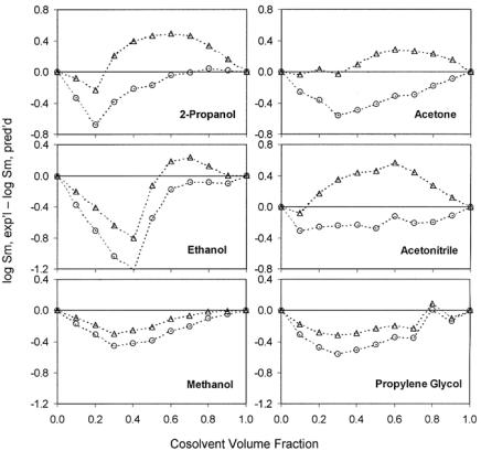
Figure 14.21.2.2c. Deviations from log-linear model (equation [14.21.2.2], triangle) and the extended log-linear model (equation [14.21.2.10], circle) for solute benzoic acid in various water cosolvent systems. Experimental data are from Refs. 61 and 86.

the UNIFAC group interaction parameters involved in these systems are incorrect. With all the systems tested in this study with solute naphthalene, benzocaine, or benzoic acid, it is also found that replacing fi in the last term of equation [14.21.2.11] with mole fraction xi offers slight improvement in only a few cases. Dropping the logarithm conversion constant 2.303 results in larger estimation errors for most systems.

An apparent limitation of this modification is the exclusion of any active role the solute may play on the observed deviation. Little understanding of the influence of solute structure and properties on deviations from the log-linear equation has been obtained. Although the patterns of deviations tend to be similar among solutes, as mentioned above, the extent of deviation is solute-dependent. For instance, C1~C4 alkyl esters of p-hydroxybenzoates and p-aminobenzoates demonstrated similar characteristics of solubilization by propylene glycol, with a negative deviation from the log-linear pattern occurring when f is low, followed by a positive one when f increases.91 The magnitude of the negative deviation, however, was found to be related to the length of the solute alkyl chain in each group, while that of the positive deviation to the type of the polar groups attached.91