

Ufimtsev P. Fundamentals of the physical theory of diffraction (Wiley 2007)(348s) PEo
.pdf2Introduction
They are also formulated in the text boxes placed at the very beginning of most chapters and sections.
Notice that PTD has found various applications. Some related references are collected at the end of the book in the Section “Additional References Related to the PTD Concept: Applications, Modifications, and Developments”. In particular, PTD was successfully used in the design of the American stealth-fighter F-117 and stealthbomber B-2 (Browne, 1991a, Browne, 1991b, Rich, 1994, Rich and Janos, 1994; see also the foreword written by Mitzner for the Ufimtsev book, 2003). The present book contains only original results obtained by the author (some of them in collaboration with colleagues).
The distinctive feature of PTD is that it belongs to the class of source-based theories. The scattered/diffracted field is considered as radiation by surface sources, which are induced (due to diffraction) on the scattering objects by the incident waves. In the case of electromagnetic waves and metallic scattering objects, these sources are the surface electric charges and currents. In the case of acoustic waves, these sources are the surface distributions of the “acoustic pressure” on rigid objects, or the surface distributions of the “fluid velocity” on soft (pressure-release) objects. The advantage of this approach, as compared to the ray-based techniques, is that it allows the calculation of the scattered field everywhere, including the diffraction regions, such as foci and caustics, where the diffracted field does not have a ray structure.
The central and original idea of PTD is the separation of surface sources into the so-called uniform and nonuniform components. This separation is a flexible procedure, based on an appropriate choice of canonical diffraction problems (Ufimtsev, 1998). In the present book (except Section 7.9), the uniform component is defined as the scattering sources induced on the infinite plane tangent to the object at a source point. In the case of incident waves with a ray structure, this component is determined according to the geometrical optics (geometrical acoustics) for electromagnetic (acoustic) waves. The field found by the integration of the uniform component is considered as a high-frequency approximation for the scattered field. In acoustic diffraction problems, this approximation is interpreted as the extended Kirchhoff approximation (KA). In electromagnetic diffraction problems, it is known as the physical optics (PO) approach. In the present book we use the term physical optics for both electromagnetic and acoustic waves, just as in the work by (Bowman et al. 1987, p. 29).
The PTD is the natural extension of PO and takes into account the additional field generated by the nonuniform component, which has a diffraction nature and is caused by any deviation of the scattering surface from an infinite tangent plane. Another definition of the uniform and nonuniform scattering sources is introduced in Section 7.9. Here, the uniform component is defined as the field induced on the halfplane tangential to the illuminated face of the scattering edge (and to the edge itself). The nonuniform component is the difference between the exact field on the tangential wedge and this new uniform component. This type of separation of the surface field allows the formulation of the advanced version of PTD, which is free from the so-called grazing singularity (Section 7.9).
TEAM LinG
Introduction 3
The localization principle related to the behavior of high-frequency diffracted fields is used to determine the asymptotic approximations for the nonuniform component. In particular, according to this principle, the nonuniform sources induced in the vicinity of sharp curved edges are asymptotically identical to the nonuniform sources induced on a tangential wedge near the tangency point.
Thus, the wedge diffraction is the basic canonical problem for the investigation of edge waves, and it is studied in detail in this book. Exact and asymptotic expressions for the 2-D edge waves are derived in Chapters 2, 3, and 4. These results are then used in Chapter 5 to construct simple asymptotic expressions for the field diffracted at strips and polygonal cylinders.
Notice that 2-D diffraction problems for acoustically soft (hard) scattering objects
are equivalent to the electromagnetic problems where the electric vector E (magnetic
vector H) is parallel to the generatrix of perfectly conducting objects. Due to this equivalence, some results obtained in Ufimtsev (1962) for 2-D electromagnetic problems are transferable for acoustic problems, with proper re-definitions of physical quantities. For the same reason, the asymptotics derived in Chapter 5 for acoustic waves are also valid for electromagnetic waves diffracted at perfectly conducting strips and trilateral cylinders.
A new physical interpretation of the classical physical optics is introduced in Chapter 1. The scattered PO field is separated into the reflected field and the shadow radiation. The first part contains the ordinary reflected rays and beams, and dominates in the geometrical optics region. The shadow radiation is equivalent to the field scattered at a black body (of the same shape and size as the actual scattering object), and dominates in the vicinity of the shadow region (Fig. 1.4, Fig. 14.6). Manifestations of the shadow radiation are the well-known phenomena Fresnel diffraction and forward scattering.
The Shadow Contour Theorem is established in Section 1.3.5, which states that different objects with identical shadow boundaries on their surfaces generate identical shadow radiation. This theorem significantly facilitates the approximate estimation of scattering at complex objects. It is also shown here that the shadow radiation contains half of the total power scattered by perfectly reflecting objects. Thus, the new formulation of the PO field elucidates the scattering physics and explains the nature of the fundamental diffraction law according to which the total scattering cross-section of large (compared to the wavelength) perfectly reflecting objects equals double the transverse area of geometrical optics shadow zone behind the object.
A significant part of this book is devoted to the theory of elementary edge waves and to its applications. The elementary edge wave is a wave radiated by surface sources, induced in the vicinity of an infinitesimal element of the edge. Highfrequency asymptotic expressions are found for the elementary edge waves and allow one to investigate the diffraction at arbitrary curved edges with large radii of curvature (as compared to the wavelength).
Elementary edge waves can also be interpreted as the elementary edge-diffracted rays. The PO field too can be understood as the linear superposition of the other type of elementary rays. Because of this, PTD can be considered as a ray theory on the level of elementary rays. Even in the diffraction regions such as geometrical optics
TEAM LinG

4Introduction
boundaries, foci, and caustics, the wave field can be represented in terms of elementary rays. The ordinary reflected and diffracted rays are found in PTD by the asymptotic evaluation of the field integrals and can be interpreted as the beams of elementary rays generated in the vicinity of the stationary points. Such a possible interpretation of PTD goes back to the intuitive Huygens principle, which was rigorously formulated by Helmholtz in terms of elementary spherical waves/rays (Bakker and Copson, 1939).
The general theory of elementary waves is applied in this book to the solution of a variety of diffraction problems. Backscattering and bistatic scattering at bodies of revolution are considered in Chapter 6. Ray and caustic asymptotics are derived in Chapter 8. Slope and multiple diffraction at large objects are investigated in Chapters 9 and 10. The results of these chapters are utilized in Chapters 11 and 12 to analyze the focusing of multiple edge waves on the symmetry axis of the bodies of revolution. The example of the disk diffraction problem (whose exact asymptotic solution is known), establishes that PTD provides correct expressions for the first term in the total asymptotic expansion for each multiple edge-diffracted wave.
Chapters 13 and 14 derive the PTD asymptotics for the field scattered at a finite cylinder under oblique incidence of a plane wave. Together with the numerical results illustrated in the figures, they explain the physical structure of the scattered field. New fine features of the theory are emphasized here. They concern the necessity to calculate the high-order terms in the PO field as well as radiation by the nonuniform component of the scattering sources caused by the smooth bending of the cylindrical surface.
The theory developed in the book can find various applications. Among them are the problems associated with the design of microwave antennas, estimation of scattering cross-sections, identification of scattering objects, propagation of waves in urban environments, and so on. In combination with numerical methods, it can be used for the development of efficient hybrid techniques for the investigation of complex diffraction problems. This book can also be useful for teaching a variety of university courses, including topics on high-frequency asymptotic techniques in diffraction theory. The problems following each chapter are intended for independent investigation and will be helpful in studying PTD, especially for students.
The International System of Units (SI) and the time dependence of exp(−iωt) for the wave fields and sources are used in this book.
ACRONYMS
GO |
Geometrical optics |
GA |
Geometrical acoustics |
GTD |
Geometrical theory of diffraction |
EEW |
Elementary edge wave |
KA |
Kirchhoff approximation |
PO |
Physical optics |
PTD |
Physical theory of diffraction |
|
|
TEAM LinG

Chapter 1
Basic Notions in Acoustic and
Electromagnetic Diffraction
Problems
1.1FORMULATION OF THE DIFFRACTION PROBLEM
This book develops the Physical Theory of Diffraction (PTD) for both acoustic and electromagnetic waves diffracted at perfectly reflecting objects.
In the case of two-dimensional (2-D) problems, this theory is valid for both electromag-
netic and acoustic waves.
First we present the theoretical fundamentals for acoustic waves and then for electromagnetic waves. In the linear approximation, the velocity potential u of harmonic acoustic waves satisfies the wave equation (Kinsler et al., 1982; Pierce, 1994)
2u + k2u = I. |
(1.1) |
Here k = 2π/λ = ω/c is the wave number, λ is the wavelength, ω the angular frequency, c the speed of sound, and I the source strength characteristic. The time dependence is assumed to be in the form exp(−iωt), and is suppressed below. The acoustic pressure p and the velocity v of fluid particles, caused by sound waves, are determined through the velocity potential (Kinsler et al., 1982; Pierce, 1994)
∂u |
= iωρu, v = u |
|
p = −ρ ∂t |
(1.2) |
where ρ is the mass density of a fluid. The power flux density of sound waves, which is the analog of the Poynting vector for electromagnetic waves, equals
P |
= |
= |
p |
|
u. |
(1.3) |
|
pv |
|
Fundamentals of the Physical Theory of Diffraction. By Pyotr Ya. Ufimtsev
Copyright © 2007 John Wiley & Sons, Inc.
5
TEAM LinG
6Chapter 1 Basic Notions in Acoustic and Electromagnetic Diffraction Problems
Its value averaged over the period of oscillations T = 2π/ω equals
av = |
2 |
|
|
P |
1 |
Re( p v). |
(1.4) |
|
Here and everywhere below, the superscript asterisk is used for complex conjugate quantities.
Two types of boundary conditions are imposed on the surface of perfectly reflecting objects: the Dirichlet condition
u = 0 or p = 0 (soft) |
(1.5) |
for objects with a soft (pressure-release) surface, and the Neumann condition
∂n |
= ˆ · |
|
= |
|
|
∂u |
n |
u |
|
0 (hard) |
(1.6) |
|
|
for objects with a hard (rigid) surface. Here u is the total field that is the sum of the incident and scattered waves. The symbol nˆ stands for a unit outward vector, which is normal to the scattering surface S (Fig. 1.1). The gradient operator is applied to coordinates of the integration /source point Q.
To complete the formulation of the diffraction problem, and to ensure the uniqueness of its solution, the above wave equation and the boundary conditions are supplemented by the Sommerfeld radiation condition for the scattered field,
lim r |
∂u |
− iku |
= 0 with r → ∞, |
(1.7) |
∂r |
where r is the distance from the scattering object to the observation point.
In the International System (SI) of units, the quantities introduced above have
the following dimensions |
|
|
|
|
|
|
|
|
|
|
|
|
||||
[r] = m, |
[t] = sec, |
|
|
[v] = [c] = |
|
m |
[ω] = |
1 |
|
|||||||
|
|
|
|
|
, |
|
, |
|||||||||
|
|
|
sec |
sec |
||||||||||||
|
kg |
|
|
kg |
|
m2 |
|
|
(1.8) |
|||||||
|
[p] = m |
[u] = |
|
|
kg |
|||||||||||
[ρ] = m3 , |
|
sec2 , |
sec , |
[P] = sec3 . |
||||||||||||
|
|
|
|
|
· |
|
|
|
|
|
|
|
|
|
|
|
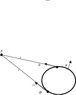
Figure 1.1 Scattering surface S. Here r is the distance between the observation point P (which can be in the far zone) and the integration point Q (on the surface of the scatterer), the unit vector mˆ is directed from the point Q to the point P.
TEAM LinG

1.2 Scattered Field in the Far Zone 7
The standard denotations are used here: m for meter, kg for kilogram, and sec for second. The pressure unit is called Pascal (Pa) and 1 Pa = 1 Newton/1 m2. The SI unit of the power flux density is 1 Watt/1 m2 = 1 Joule/(1 sec · 1 m2).
In the scattering problems, which admit the electromagnetic interpretation, the quantity u plays the role of the electric field intensity ([E] = Volt/m) or magnetic field intensity ([H] = Ampere/m), depending on the polarization of electromagnetic waves. Their power flux density is called the Poynting vector and is defined as
|
= |
× |
av = |
2 |
[ |
× |
|
] |
|
|
P |
E |
H |
and P |
1 |
Re E |
H |
|
|
. |
(1.9) |
|
|
1.2SCATTERED FIELD IN THE FAR ZONE
The scattered field is determined by the Helmholtz integral expressions (Bakker and Copson, 1939):
us = − |
1 |
∂u eikr |
ds, |
uh = |
1 |
S u |
∂ |
eikr |
ds, |
(1.10) |
||||
|
|
|
|
|
|
|
|
|
||||||
4π |
S ∂n r |
4π |
∂n |
|
r |
|||||||||
where the integrals are taken over the scattering surface S. The function us describes the field scattered by an acoustically soft object, and the function uh relates to the field scattered by an acoustically hard object. The field quantities u and ∂u/∂n in the integrands belong to the total field on the object surface, that is, to the sum of the incident and scattered fields. These quantities represent the surface sources of the scattered field induced by the incident wave. We denote them by symbols
js = |
∂u |
|
∂n , jh = u, |
(1.11) |
similar to those used for induced sources/currents in the electromagnetic version of PTD (Ufimtsev, 2003). The quantity eikr /r in Equation (1.10) represents the Green function of a homogeneous medium, that is, the fundamental solution of the wave equation, and nˆ is a unit outward vector normal to the surface S.
In the far field, where r kd2 (d is the characteristic linear dimension of the object), the field expressions (1.10) can be simplified. We choose the origin of the coordinate system somewhere inside the object, as shown in Figure 1.2. Under the
conditions R |
r , R |
kd2, we have |
|
|
|
|
|
|
|
|
|||||
|
|
|
|
|
|
|
|
|
|
ikr |
|
ikR |
|
|
|
|
|
|
|
|
r ≈ R − r cos , |
|
|
e |
≈ |
e |
e−ikr cos |
(1.12) |
|||
|
|
|
|
|
|
|
r |
R |
|||||||
with |
|
|
|
|
|
|
|
|
|
|
|
|
|
|
|
|
|
|
|
cos = cos ϑ cos ϑ + sin ϑ sin ϑ cos(ϕ − ϕ ). |
(1.13) |
||||||||||
In addition, |
|
|
|
|
|
|
|
|
|
|
|
|
|||
|
∂ |
eikr |
|
eikr |
1 |
|
eikr |
|
|
|
|
||||
|
|
|
|
= |
|
· nˆ = − ik − |
|
|
|
|
r · nˆ , |
with r = mˆ , |
(1.14) |
||
|
∂n |
|
r |
r |
r |
|
r |
||||||||
TEAM LinG
8Chapter 1 Basic Notions in Acoustic and Electromagnetic Diffraction Problems
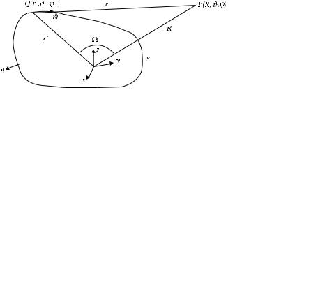
Figure 1.2 S is the surface of the scattering object; Q is the integration point (with the spherical coordinates r , ϑ , ϕ ) on the surface S; P is the observation point (with the coordinates R, ϑ , ϕ) in the far zone; is the angle between the directions from the origin to the integration and observation points.
or in view of Equations (1.12)
∂ |
|
eikr |
≈ − |
ik |
eikR |
e−ikr cos |
· |
(m |
n). |
(1.15) |
∂n |
|
r |
|
|||||||
|
|
R |
ˆ |
· ˆ |
|
|||||
Finally, we obtain the following approximations for the field in the far-away point P:
us = − |
1 |
|
eikR |
S jse− |
ikr |
cos |
ds, |
|
(1.16) |
|
4π |
|
R |
|
|
|
|||||
uh |
= − |
ik |
|
eikR |
jhe−ikr cos (m |
n)ds |
(1.17) |
|||
|
|
|
||||||||
|
4π |
|
R |
S |
|
|
ˆ |
· ˆ |
|
|
where mˆ and nˆ are unit vectors. In this book, we develop asymptotic approximations first for the surface sources js,h and then for the scattered field (1.16), (1.17).
Expressions (1.16) and (1.17) can be written in the generic form
|
|
|
|
|
us,h = u0 s,h |
eikR |
|
|
|
(1.18) |
||||
|
|
|
|
|
R |
|
|
|
|
|
|
|||
where the functions |
|
|
|
|
|
|
|
|
|
|
|
|||
|
s = − |
1 |
|
j |
e−ikr cos ds, |
|
|
|
ik |
|
j |
e−ikr |
cos (m |
n)ds |
4π u0 S |
|
4π u0 S |
||||||||||||
|
s |
|
h = − |
h |
|
ˆ |
· ˆ |
|||||||
|
|
|
|
|
|
|
|
|
|
|
|
|
|
(1.19) |
represent the directivity patterns of the scattered field, and u0 is the complex amplitude of the incident wave at the origin of the coordinates (R = 0). Notice that in the vicinity of the scattering object located in the far zone from the source Q , the incident wave can be approximated by the equivalent plane wave with the amplitude u0.
TEAM LinG

1.2 Scattered Field in the Far Zone 9
According to Equations (1.2), (1.3) and (1.4), the power flux density of the scattered field is determined by
Psc = iωρu u. |
(1.20) |
|
In the far field, |
|
|
u ≈ iku · Rˆ , |
with Rˆ = R. |
(1.21) |
Therefore, the power flux density averaged over the oscillation period T = 2π/ω equals
av = |
2 |
|
[ |
] = |
2 |
[ |
|
] · ˆ |
= |
2 |
| |
| |
|
· ˆ |
|
|
Psc |
|
1 |
Re |
|
p v |
1 |
Re |
(iωρu) (iku) |
R |
|
1 |
k2Z |
u |
2 |
R, |
(1.22) |
|
|
|
|
|
|
|
||||||||||
where |
|
|
|
|
|
|
|
|
|
|
|
|
|
|
|
|
|
|
|
|
|
|
|
Z = ρc |
|
|
|
|
|
|
|
(1.23) |
|
is the characteristic impedance of the medium.
Usually, the far field is characterized by the bistatic cross-section σ introduced through the relation
Pavsc |
= |
σ · Pavinc |
, |
|
(1.24) |
|||||
|
|
4π R2 |
|
|
|
|||||
where |
|
|
|
|
|
|
|
|
|
|
inc |
|
|
1 |
|
2 |
|
inc |
2 |
|
|
Pav |
= |
|
k |
|
Z|u |
|
| |
|
(1.25) |
|
2 |
|
|
|
|||||||
is the power flux density of the incident wave. This definition suggests the interpretation given in the following paragraphs.
The bistatic cross-section is the area σ of a hypothetical plate perpendicular to the direction of the incident wave. This plate intercepts the incident power Pavinc · σ and distributes it uniformly into the whole surrounding space with the power flux density that is equal to the actual one scattered by the object in the direction of observation. Because the scattered power depends on the direction of scattering, the scattering cross-section σ is a function of this direction. The term bistatic means that the direction of scattering can be arbitrary. In the particular case when the scattering direction coincides with the direction to the source of the incident wave, the quantity σ is called the backscattering cross-section or monostatic cross-section. Thus, according to Equations (1.22) and (1.24)
σ |
|
4π R2 |
Pavsc |
|
4π R2 |
|usc|2 |
. |
(1.26) |
= |
Pavinc = |
|
||||||
|
|
|uinc|2 |
|
|||||
In the directions where the field scattered from a smooth convex surface has a ray structure, the bistatic cross-section is predicted by Geometrical Optics (Geometrical
TEAM LinG
10 Chapter 1 Basic Notions in Acoustic and Electromagnetic Diffraction Problems
Acoustics) and equals
σ = πρ1ρ2. |
(1.27) |
Here ρ1 and ρ2 are principal radii of curvature of the scattering surface at the reflection point. It is also assumed that this surface is perfectly reflecting (soft or hard). Two interesting features of this quantity should be emphasized.
First, the expression (1.27) is universal. It is applicable both for acoustic and electromagnetic waves. The reason for this is that the ray structure does not depend on the nature of the waves, and it is totally determined by the geometry of the scattering surface. If the geometry is the same, the divergence of reflected rays will be the same for both acoustic and electromagnetic rays. Also, the modulus of reflection coefficient for any perfectly reflecting surfaces (soft or hard for acoustic waves, or perfectly conducting for electromagnetic waves) equals unity. However, just these two factors, the ray divergence and the reflection coefficient, totally determine the amplitude of reflected rays, and eventually the bistatic cross-section.
Equation (1.27) can be generalized for imperfect reflecting surfaces:
σ = |R|2πρ1ρ2, |
(1.28) |
where R is the reflection coefficient, which can be different for acoustic and electromagnetic waves.
The second interesting and not obvious feature of Equation (1.27) is the following. This expression does not depend on the angle between the incident and reflected rays at the same reflection point (Fig. 1.3). In other words, it is constant for any bistatic angles, including zero angle related to backscattering. This property of scattering from perfectly reflecting objects follows from the theory of Fock (1965) as it was shown in Ufimtsev (1999).
The theory of Fock (1965) is more general. It is also valid for imperfect scattering surfaces characterized by the reflection coefficient R. In this case, Fock’s theory leads straight to Equation (1.28), where R depends on the bistatic angle as well as on the boundary conditions.
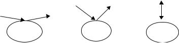
Figure 1.3 Scattering from the same reflection point (at the same reflecting object) for
different bistatic angles. Bistatic cross-section σ of this perfectly reflecting object is constant for all of these angles and equals the monostatic cross-section.
TEAM LinG

1.3 Physical Optics 11
1.3PHYSICAL OPTICS
This high-frequency approach is widely used in acoustic and electromagnetic diffraction
problems.
1.3.1Definition of the Physical Optics
Physical Optics (PO) was suggested by Macdonald (1912), and since then it has been successfully applied in the theory of diffraction. In particular it is often used in the analysis of electromagnetic waves scattered from large metallic objects. Basic features of this approach in the study of electromagnetic diffraction are exposed in the article by Ufimtsev (1999). The scalar version of PO is applicable for acoustic waves and it is known in acoustics as the extended Kirchhoff approximation (Brill and Gaunaurd, 1993; Menounou et al., 2000; Moser et al., 1993). Physical Optics is a constituent part of the Physical Theory of Diffraction developed in the present book. According to this approximation, the field induced on the surface of the object is determined by Geometrical Optics (Geometrical Acoustics).
The physics behind this is as follows. Geometrical Optics describes a wave field in the limiting case when a wavelength tends to zero. With respect to such a small wavelength, the scattering surface at the reflection point can be considered approximately as a tangential plane. Therefore, the surface field induced at the tangential infinite plane is a good high-frequency approximation for true scattering sources induced on a large scattering object. Two such planes P1 and P2 tangent at the points Q1 and Q2 are shown in Figure 1.4. These points are located at the “illuminated” side of the object. Notice that according to Geometrical Optics, the field equals zero in the shadow region, including the points on the object surface.
Thus, the reflection from a tangential plane is an appropriate canonical (“fundamental”) problem. Its exact solution can be easily found using Geometrical Optics, as well as by image theory. The total field generated by an external source above an infinite reflecting plane (Fig. 1.5) is the sum of the incident field and the reflected field, which can be interpreted as the field created by the image source. On the acoustically soft plane, the total field is zero as a result of the boundary condition (1.5), but its normal derivative equals
∂us |
|
∂uinc |
|
|
= 2 |
s |
(1.29) |
∂n |
∂n |
due to the exact solution of this problem. On the acoustically hard plane, the normal derivative of the total field is zero as a result of the boundary condition (1.6), and the field itself equals
uh = 2uhinc, |
(1.30) |
TEAM LinG