Ufimtsev P. Fundamentals of the physical theory of diffraction (Wiley 2007)(348s) PEo

262 Chapter 12 Focusing of Multiple Edge Waves Diffracted at a Disk

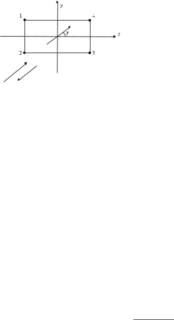
Figure 12.1 Disk projection on the plane y0z (bold solid lines) and the edge waves (dashed lines). Angles ϕ and ψ = 2π − ϕ (measured from the left and right faces of the disk) determine the directions to the observation point P.

determined by Equation (11.3) adjusted to the disk problem as

Here, a is the radius of the disk, ψ = 2π − ϕ, α = 2π . The quantity u¯l(m,t) is the total m-order edge wave arrived along the left face of the disk to the edge point ζ ,

¯ (m,t) = ¯ (m) + ¯(m)

ul ull url . (12.4)

¯ (m)

The quantity ull denotes the m-order wave on the left face (at the edge point ζ )

¯ (m)

at the edge along the left face. Analogously, the quantity url is the m-order wave on the left face (at the point ζ of the edge) generated (at the point ζ − π a) by the

denotations the sense of the following function becomes clear

¯ (1,t) ≡ ¯ pr ¯ (1,t) ≡ ¯ pr

The quantities ul ul and ur ur are the primary edge waves at the disk face, which passed through the focal line and arrived at the edge point ζ . They can be

found with application of Equation (8.29), where one should set γ0 = π/2, R = 2a, ρ = −a, and g = g(0, π/2, α) for u¯lpr , and g = g(α, π/2, α) for u¯rpr . In the same way

¯(m) ¯ (m) ¯ (m) =

one can find the quantities ull , ulr , url with m 2, 3, . . . ; only the function g will be different, namely g = g(0, 0, α) = −1. We omit all intermediate manipulations and obtains the results:

The function g(ϕ, π/2, α) is singular in the directions ϕ = π/2 and ϕ = 3π/2. Because of this, the total scattered field in the far zone should be represented in the traditional PTD form:

TEAM LinG

264 Chapter 12 Focusing of Multiple Edge Waves Diffracted at a Disk

with g(1)(π/2, π/2, α) = −g(3π/2, π/2, α) = −1/2, is the field generated by the nonuniform/fringe scattering sources jh(1) caused by the primary diffraction of the incident wave at the disk. The series in Equations (12.14) and (12.15) represent the contributions generated by that part of jh(1) that is caused by the multiple diffraction.

After the substitution of Equation (12.15) into Equation (11.8) one finds the total

This is the incomplete asymptotic approximation, which includes only the first term of the total asymptotic expansion (with ka → ∞) for each multiple edge wave. Comparison with the exact asymptotic solution (Witte and Westpfahl, 1970), which contains six first terms for the total cross-section, confirms that Equation (12.18) is correct.

12.2MULTIPLE SOFT DIFFRACTION

The focal field created by the primary edge waves (excited by the incident wave uinc = exp(ikz)) is determined according to Equation (11.2) as

This is the edge wave generated by the total scattering sources j stot = js(0) + js(1). The focal field of the primary edge waves created only by the nonuniform component js(1) is also described by Equation (12.1), where one should replace the function f by

TEAM LinG

12.2 Multiple Soft Diffraction 265

The higher-order edge waves arise due to the slope diffraction of waves running along the flat faces of the disk. They are calculated on the basis of Equation (10.19). In the case of diffraction at a solid convex body of revolution, the related technique was developed in Section 11.2. In the present section, this technique is extended for the investigation of diffraction at an acoustically soft disk. According to Equation (10.19),

of the problem is shown in Figure 12.1. The angles ϕ and ψ are measured from different faces of the disk and ψ = 2π − ϕ. Due to the axial symmetry of the problem, Equation (12.23) is reduced to

¯ (m,t)

Here, ul,r is the amplitude factor of the wave, which is equivalent to the total

along the left or right face, as indicated by the subscripts l, r. In accordance with Equation (12.1) the scattered field is also symmetric with respect to the disk plane, therefore

¯(m)

consists of two equal terms. The term ull relates to the m-order edge wave on the left face of the disk at the point ζ . This wave is generated by the (m − 1)-order edge wave

TEAM LinG

266 Chapter 12 Focusing of Multiple Edge Waves Diffracted at a Disk

and arrived there along the right side of the disk. Because of the symmetry of the field, these terms are equal to each other.

¯(m) ¯ (m,t)

The quantities ull and ul are calculated with application of Equations (10.18) and (10.20), where one should set γ0 = γ01 = π/2, R = 2a, and ρ = −a. These calculations result in

¯(1,t) = ¯ (1)

The denotation ul ul is used to emphasize that only one primary edge wave exists on each side of the disk, but two edge waves of any higher order are on every side. Thus,

This expression can be used to calculate the total cross-section (11.8), where ustot is the total field scattered in the forward direction ϕ = 3π/2. In the present case,

TEAM LinG

12.3 Multiple Diffraction of Electromagnetic Waves 267

The substitution of Equation (12.35) into Equation (11.8) determines the total crosssection

This is the incomplete asymptotic expression, which includes only the first term of the total asymptotic expansion for every edge wave. It can be verified by comparison with the exact asymptotic expression (14.54) in Bowman et al. (1987), which contains the asymptotic terms up to the order of (ka)−4. According to Equation (12.37),

All these three terms are identical to the exact ones. Thus, the comparison of asymptotics (12.18) and (12.37) with known exact results proves that PTD correctly predicts the first term in the total asymptotic expansion for every multiple edge wave.

12.3 MULTIPLE DIFFRACTION OF ELECTROMAGNETIC WAVES

at a perfectly conducting disk (Fig. 12.1). The basic features of this problem are essentially the same as those in the acoustical problems above. For this reason, we will not repeat them here and only briefly discuss a new specific feature caused by the vector nature of electromagnetic waves. Due to this nature and to the axial symmetry of the problem, one can separate the diffracted waves (of the second and higher orders) into two independent groups, with Eϕ - and Hϕ -polarizations. Multiple diffraction of the Eϕ -waves (Hϕ -waves) is calculated just like the diffraction of acoustic waves at a soft (hard) disk. This observation significantly facilitates the investigation, which results in the following approximations for the focal field on the z-axis (z kR2). The focal fields generated by all the multiple Eϕ -waves and Hϕ -waves are equal to

TEAM LinG

268 Chapter 12 Focusing of Multiple Edge Waves Diffracted at a Disk

The focal field includes these fields plus the contributions generated by the current

j(0) (PO contribution) and the current j(1) (related to the primary edge diffraction):

Now, according to Equation (11.8), which is also valid for electromagnetic waves (with the replacement of u(t) by Ex(t)), one obtains the total scattering cross-section:

with the similar quantities (11.9) and (11.18) found for acoustic waves.

PROBLEMS

12.1Prove Equation (12.14) for the focal field generated by all of the acoustic edge waves scattered at a hard disk. Explain all of the details, including caustic parameters, phase shifts, directivity factors, and fractional coefficients.

12.2Prove Equation (12.34) for the focal field generated by all of the acoustic edge waves scattered at a soft disk. Explain all of the details, including caustic parameters, phase shifts, directivity factors, and fractional coefficients.

12.3Prove Equation (12.40) for the focal field generated by the Eϕ -group of the electromagnetic edge waves scattered at a perfectly conducting disk. Explain all of the details, including caustic parameters, phase shifts, directivity factors, and fractional coefficients.

12.4Prove Equation (12.41) for the focal field generated by the Hϕ -group of the electromagnetic edge waves scattered at a perfectly conducting disk. Explain all of the details, including caustic parameters, phase shifts, directivity factors, and fractional coefficients.

TEAM LinG