


Ref. p. 131] |
|
|
|
|
|
|
|
|
3.1 Linear optics |
127 |
||||||||||
|
|
|
|
|
|
|
|
|
|
|
||||||||||
The result is an output Gaussian intensity distribution with the waist radius |
|
|||||||||||||||||||
w O = |
|
|
w I |
|
|
, |
|
|
|
|
|
|
|
|
|
|
|
|
|
|
|
|
|
|
|
|
|
|
|
|
|
|
|
|
|
|
|
|
|
||
1 + |
w2 |
|
2 |
|
|
|
|
|
|
|
|
|
|
|
|
|
||||
|
π I |
|
|
|
|
|
|
|
|
|
|
|
|
|
|
|
||||
|
λ f |
|
|
|
|
|
|
|
|
|
|
|
|
|
|
|
||||
|
|
|
|
|
|
|
|
|
π w O w I |
|
2 |
|
|
|
|
|
|
|
|
|
the waist position z = zwaist = f |
, and z O = |
π w2O/λ . |
|
|||||||||||||||||
λ f |
|
|||||||||||||||||||
For inclusion of displacements and misalignments in Collins Integral see [96Tov]. |
|
|||||||||||||||||||
3.1.7.4.2 Three-dimensional propagation |
|
|
|
|
|
|
|
|
||||||||||||
In Table 3.1.23 the propagation in in general astigmatic systems is given. |
|
|||||||||||||||||||
Table 3.1.23. Propagation in general astigmatic systems. |
|
|
||||||||||||||||||
|
|
|
|
|
|
|
|
|
|
|
|
|
|
|
|
|
|
|
|
|
Given |
|
|
|
|
|
|
|
Solution |
|
|
|
|
|
|
|
|
|
|
|
|
|
|
|
|
|
|
|
|
|
|
|||||||||||
– S : matrix of |
the optical sys- |
Field U O(r2) in the output plane (Collins integral ): |
|
|||||||||||||||||
tem, see Table 3.1.15 and |
|
|
|
|
− |
i exp(−i kL) |
|
|
|
|||||||||||
(3.1.99) with |
|
|
|
|
|
|
U O(r2) = |
|
|
d r1U I (r1) |
|
|||||||||
|
|
|
|
|
|
|
|
|
|
|
|
λ |
√ |
det B |
|
|
|
|||
|
A B |
|
|
|
|
|
|
|
|
|
|
k |
|
|
|
|
|
|
||
S = C D |
, |
|
|
|
|
× exp −i |
|
|
r1 B−1 A r1 − 2 r1 B−1 r2 + r2 D B−1 r2 |
(3.1.132) |
||||||||||
|
|
|
|
2 |
|
|||||||||||||||
– field distribution in the input |
with det B the determinant and B−1 the inverse of the matrix B . |
|||||||||||||||||||
plane: U I(r1) , where r1 is the |
Examples in [70Col, 05Gro2, 05Hod]. |
|
||||||||||||||||||
position vector in the input |
|
|
|
|
|
|
|
|
|
|
|
|
|
|||||||
plane. |
|
|
|
|
|
|
|
|
|
|
|
|
|
|
|
|
|
|
|
|
|
|
|
|
|
|
|
|
|
|
|
|
|
|
|
|
|
|
|
|
|
3.1.7.5Gaussian beams in optical systems with stops, aberrations, and waveguide coupling
3.1.7.5.1Field distributions in the waist region of Gaussian beams including stops and wave aberrations by optical system
Classical cases of optical system design are given in [99Bor, 80Hof, 86Haf]. [82Wag, 95Gae] use the calculation of the field distribution in the image by a stop and wave aberrations in the exit pupil.
The analog is modeled for Gaussian beams on the exit pupil in the following references:
–focused Gaussian beams with aberrations and stops: see [69Cam, 71Sch],
–obscuration of a rotationally symmetrical Gaussian beam including longitudinal focal shift: see [82Car, 86Sta],
–extended systematic discussion of di raction with stops, obscuration, and aberrations: see [86Mah, 01Mah],
–spherical aberration: see [98Pu].
Landolt-B¨ornstein
New Series VIII/1A1

128 |
3.1.7 Beam propagation in optical systems |
[Ref. p. 131 |
|
|
|
3.1.7.5.2 Mode matching for beam coupling into waveguides
The calculation of the excitation coe cient of an eigenmode in a waveguide (output mode) by the incident mode (input mode) at the surface of the waveguide is described in Table 3.1.24.
This task occurs
–if a laser beam is formed by an optical system and coupled afterwards into an optical fiber,
–if a laser beam of a master oscillator is to be coupled into a power amplifier,
–in the case of waveguide-waveguide coupling especially fiber-fiber coupling or coupling between semiconductor lasers.
Solutions are available in commercial optical design programs.
Table 3.1.24. Definitions for waveguide coupling.
Given |
Solution |
|
|||
|
|
|
|
|
|
– |
Incident beam (emitted by a laser |
Coupling coe cient (power relation): |
|
||
|
(and) transformed by an optical system): |
|
O IO O IO |
|
|
|
Einput (x, y) . |
η = |
. |
(3.1.133) |
|
|
|
||||
– |
Waveguide with an eigenmode field the |
|
N I N O |
|
|
|
coupling to which is asked: Eoutput (x, y) . |
Overlap integral : |
|
||
Plane of mode |
O IO = |
∞ |
∞ |
(3.1.134) |
|||
x |
|
|
d x |
d y E I(x, y) E O(x, y) . |
|||
matching |
|
|
|
|
|
|
|
|
|
|
−∞ |
−∞ |
|
||
Einput ( x) |
Eoutput ( x) |
Normalization: |
|
|
|||
z |
|
∞ |
∞ |
|
|
||
|
|
N I = |
|
d x |
d y E I(x, y) E I (x, y) . |
(3.1.135) |
|
|
Waveguide |
|
−∞ |
−∞ |
|
|
|
Fig. 3.1.44. Mode matching. |
Normalization: |
|
|
||||
Asked: Part of power transmitted into the waveguide (fiber, laser, integrated optical waveguide).
∞ |
∞ |
|
|
|
|
N O = |
d x d y E O(x, y) E O(x, y) . |
(3.1.136) |
−∞ |
−∞ |
|
E ective antireflection layers are assumed to be on the waveguide.
3.1.7.5.3 Free-space coupling of Gaussian modes
For the case that a Gaussian output waist of a source waveguide and a Gaussian input waist of a receiver waveguide are separated by air, the coupling of both waveguides is generally treated in [64Kog]. Higher-order modes are also included. The approximation of small misalignments (o set and tilt) is given in Table 3.1.25, large o sets and tilts are treated in [64Kog, 91Wu].
Landolt-B¨ornstein
New Series VIII/1A1
Ref. p. 131] |
|
|
3.1 Linear optics |
|
|
|
|
|
|
|
|
|
|
129 |
||||||||
|
|
|
|
|
|
|
|
|
|
|
|
|
|
|
|
|
|
|
|
|||
Table 3.1.25. Coupling of waveguides . |
|
|
|
|
|
|
|
|
|
|
|
|
|
|
|
|
|
|
|
|||
|
|
|
|
|
|
|
|
|
|
|
|
|
|
|
|
|
|
|
|
|
|
|
Given |
|
|
Solution |
|
|
|
|
|
|
|
|
|
|
|
|
|
|
|
|
|
|
|
|
|
|
|
|
|
|
|
|
|
|
|
|
|
|
|
|
|
|
|
|
|
|
– |
Source WG1 (laser, |
waveguide) which |
|
|
|
|
|
|
|
|
4 |
|
|
|
|
|
|
|
|
|
|
|
|
emits a Hermite-Gaussian beam, |
η 00−00 = |
|
|
|
|
|
|
|
|
|
|
|
|
|
|
|
|
|
|||
|
2 |
|
π w I w O |
2 |
1 |
|
|
1 |
|
|
2 |
|||||||||||
|
receiver WG2 (laser, waveguide) which can |
|
|
w I w O |
|
|
|
|
|
|
|
|||||||||||
– |
|
|
|
+ |
|
+ |
|
|
|
|
|
|
− |
|
|
|
|
|||||
accept Hermite-Gaussian eigenmodes: |
|
|
w O |
w I |
|
λ |
|
|
R I |
R O |
|
|||||||||||
|
|
|
|
− |
8 (w 0 I w 0 O ∆ x)2 |
|
k2 ψ2 |
|
2 |
|
2 |
|
|
|
|
|
||||||
|
|
|
|
(w20 I + w20 O)3 |
− |
2 |
|
|
|
|
|
|
|
|
||||||||
|
Plane of coupling |
|
|
|
|
|
|
|
|
|
|
|
w I + w O . |
|
|
|
||||||
|
R O |
|
|
|
|
|
|
|
|
|
|
|
|
|
|
|
|
(3.1.137) |
||||
|
|
w0O |
|
|
|
|
|
|
|
|
|
|
|
|
|
|
|
|
|
|
|
|
|
w |
O |
|
|
|
|
|
|
|
|
|
|
|
|
|
|
|
|
|
|
|
|
|
|
|
|
|
|
|
|
|
|
|
|
|
|
|
|
|
|
|
|
|
|
|
w0I |
|
x |
WG1 |
w I |
WG2 |
R I
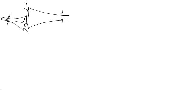
Fig. 3.1.45. Coupling of Gaussian beams. w 0 I and w 0 O: beam waist radii for WG1 and WG2, respectively; w I and w O : beam radii in the coupling plane; R I and R O: curvature radii of the beam wavefronts in the coupling plane; k = 2 π/λ ; λ : the wavelength of light; ∆ x : the lateral o set between the waveguides; ψ : the tilt of the axis.
Asked : The e ciency of the excitation of the modes in WG2, here the fundamental mode 00.
η 00−00 = 1 for ∆ x = ψ = 0 and the exact beam radii and curvature fitting w I = w O and R I = R O , otherwise
η 00−00 < 1 .
Equation (3.1.137) contains the approximations:
–Gaussian beams (paraxial optics).
–Right-hand side of (3.1.137): 2nd and 3rd term 1st term.
About coupling coe cients for higher-order modes and without the approximation: see [64Kog]; on couplings with Hermite-Gaussian modes and Laguerre-Gaussian modes: see [94Kri, 80Gra].
3.1.7.5.4 Laser fiber coupling
Methods of treatment:
–Launching of fundamental-mode laser radiation into the fundamental mode of a single-mode fiber:
–Calculation of the overlap integral (3.1.134) for a Gaussian mode and the mode field for di erent fiber cross sections: see [88Neu, p. 179], [80Gra].
–Approximation of the exact fiber fundamental modes by a Gaussian field distribution (see [88Neu, pp. 68]) and the application of the waist transformation from laser via an optical system with the methods of Sects. 3.1.7.2–3.1.7.4 and calculation of the overlap integral equation (3.1.134) or mode-coupling equation (3.1.137) [91Wu].
–Launching of fundamental-mode laser radiation or multimode laser radiation or incoherent light sources into multimode fibers:
–Overlap integral techniques in the framework of partial coherence theory: see [87Hil].
–Geometric optical methods (ray tracing and phase space techniques): see [90Gec, 95Sny, 91Gra, 91Wu, 01I ].
Landolt-B¨ornstein
New Series VIII/1A1
130 |
3.1.7 Beam propagation in optical systems |
[Ref. p. 131 |
|
|
|
–Inclusion of the aberrations and stops of the optical system used:
–Monomodal and partial coherent case: calculation of the wave aberrations of the optical system by ray-tracing methods and inclusion of these aberrations into the overlap integral: see [82Wag, 95Gae, 89Hil, 99Gue].
–Ray-tracing methods are adequate for stops and aberrations, but not reliable for a few mode waveguides: rough design [01I ]: the spot diagram of the ray tracing in the fiber facet should be within the core area and the angles of incidence should be smaller then the aperture angle [88Neu] of the fiber.