

1Foundation of Mathematical Biology / The Elements of Statistical Learning
.pdfProstate Cancer Example
Subjects: 97 potential radical prostatectomy pts
Outcome: log prostate specific antigen ( lpsa)
Covariates: log cancer volume (lcavol), log prostate weight (lweight), age, log amount of benign hyperplasia (lbph), seminal vesicule invasion (svi), Gleason score (gleason), log capsular penetration (lcp), percent Gleason scores 4 or 5 (pgg45).
Term |
Value StdError tvalue Pr(>|t|) |
|||
Intercept |
0.6694 |
1.2964 |
0.5164 |
0.6069 |
lcavol |
0.5870 |
0.0879 |
6.6768 |
0.0000 |
lweight |
0.4545 |
0.1700 |
2.6731 |
0.0090 |
age -0.0196 |
0.0112 |
-1.7576 |
0.0823 |
|
lbph |
0.1071 |
0.0584 |
1.8316 |
0.0704 |
svi |
0.7662 |
0.2443 |
3.1360 |
0.0023 |
lcp -0.1055 |
0.0910 |
-1.1589 |
0.2496 |
|
gleason |
0.0451 |
0.1575 |
0.2866 |
0.7751 |
pgg45 |
0.0045 |
0.0044 |
1.0236 |
0.3089 |
Prostate Cancer: Correlation Matrix
|
lcv |
lwt |
age |
lbh |
svi |
lcp |
gle |
pgg lpsa |
|
lcavol |
1.00 |
0.194 |
0.2 |
0.027 |
0.54 |
0.675 |
0.432 |
0.43 |
0.7 |
lweight |
0.19 |
1.000 |
0.3 |
0.435 |
0.11 |
0.100 |
-0.001 0.05 |
0.4 |
|
age |
0.22 |
0.308 |
1.0 |
0.350 |
0.12 |
0.128 |
0.269 |
0.28 |
0.2 |
lbph |
0.03 |
0.435 |
0.4 |
1.000 |
-0.09 -0.007 |
0.078 |
0.08 |
0.2 |
|
svi |
0.54 |
0.109 |
0.1 |
-0.086 |
1.00 |
0.673 |
0.320 |
0.46 |
0.6 |
lcp |
0.68 |
0.100 |
0.1 |
-0.007 |
0.67 |
1.000 |
0.515 |
0.63 |
0.5 |
gleason |
0.43 |
-0.001 |
0.3 |
0.078 |
0.32 |
0.515 |
1.000 |
0.75 |
0.4 |
pgg45 |
0.43 |
0.051 |
0.3 |
0.078 |
0.46 |
0.632 |
0.752 |
1.00 |
0.4 |
lpsa |
0.73 |
0.354 |
0.2 |
0.180 |
0.57 |
0.549 |
0.369 |
0.42 |
1.0 |
Prostate Cancer: Forward Stepwise Selection
|
lcavol lweight age lbph svi lcp gleason pgg45 |
|||||||
1 |
T |
F |
F |
F |
F |
F |
F |
F |
2 |
T |
T |
F |
F |
F |
F |
F |
F |
3 |
T |
T |
F |
F |
T |
F |
F |
F |
4 |
T |
T |
F |
T |
T |
F |
F |
F |
5 |
T |
T |
T |
T |
T |
F |
F |
F |
6 |
T |
T |
T |
T |
T |
F |
F |
T |
7 |
T |
T |
T |
T |
T |
T |
F |
T |
8 |
T |
T |
T |
T |
T |
T |
T |
T |
Residual sum of squares: |
|
|
|
|
|||
1 |
2 |
3 |
4 |
5 |
6 |
7 |
8 |
58.952.9 47.7 46.4 45.5 44.8 44.2 44.1
F-statistics for inclusion:
1 |
2 |
3 |
4 |
5 |
6 |
7 |
8 |
111.2 10.5 10.0 2.5 1.9 1.3 1.3 0.1
Prostate Cancer: Forward Stepwise Selection
|
• |
|
|
|
|
55 |
|
|
|
residual sum of squares |
• |
|
|
|
50 |
|
|
|
|
|
|
• |
|
|
|
|
• |
|
|
|
45 |
|
• |
|
|
|
• |
|
|
|
|
|
• |
• |
|
2 |
4 |
6 |
8 |
|
|
|
size |
|

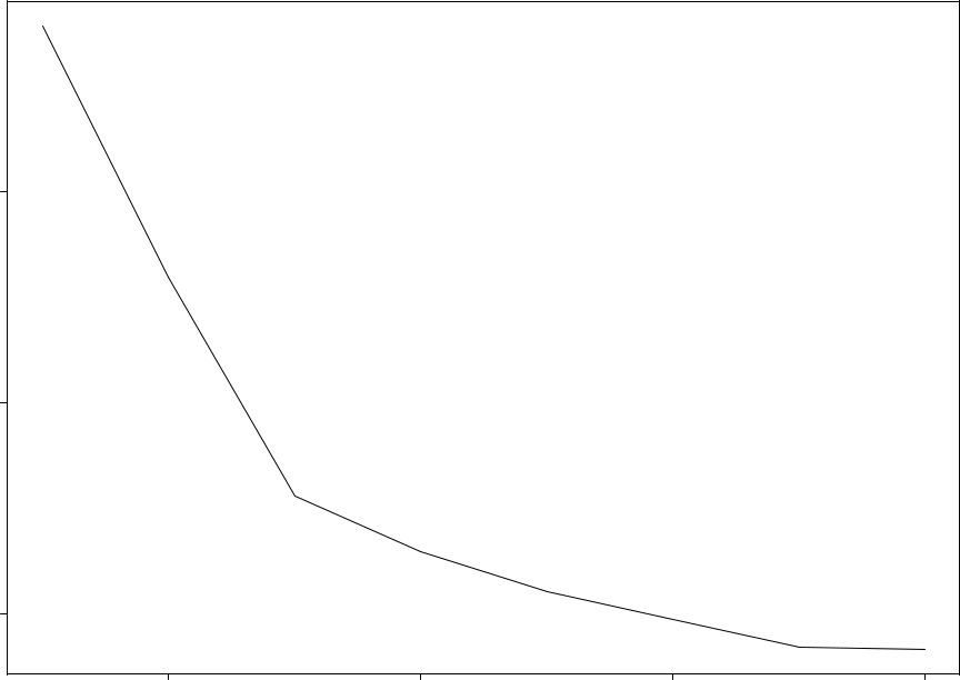
Prostate Cancer: Backward Stepwise Selection
|
• |
|
|
|
|
|
|
|
120 |
|
|
|
|
|
|
squares |
100 |
|
|
|
|
|
|
residual sum of |
80 |
|
|
|
|
|
|
|
60 |
• |
|
|
|
|
|
|
|
|
|
|
|
|
|
|
|
• |
|
|
|
|
|
|
|
|
• |
• |
• |
• |
|
|
|
|
|
• |
|||
|
|
|
|
|
|||
|
0 |
2 |
|
4 |
|
6 |
|
|
|
|
|
size |
|
|
|
Coefficient Shrinkage (Secn 3.4)
Selection procedures interpretable. But – due to in / out nature – variable ) high prediction error. Shrinkage continuous: reduces prediction error.
Ridge Regression: shrinks coefs by penalizing size:
β |
|
arg min |
|
N |
|
p |
βjxi j) |
p |
βj ) |
ridge = |
|
∑(yi β0 ∑ |
+ λ ∑ |
||||||
ˆ |
|
|
|
|
|
2 |
|
2 |
|
|
|
β |
( |
i=1 |
|
j=1 |
|
j=1 |
|
|
|
|
|
|
|
|
|||
Center X : xi j |
xi j x¯j |
ˆ |
= y¯) X |
N p. |
|||||
(β0 |
|||||||||
Minimize |
RSS(β; λ) = (y Xβ)T (y Xβ)+ λβT β |
||
Solution |
ˆ ridge = ( |
T |
1 T |
β |
X X + λI) |
X y |
|
Now nonsingular even if XT X not full rank. Interpretation via SVD: pp 60 - 63.
Choice of λ?? Microarray applications??
Coefficient Shrinkage ctd (Secn 3.4)
The Lasso: like ridge but with L1 penalty:
β |
|
arg min |
|
N |
p |
βjxi j) |
p |
lasso = |
|
∑(yi β0 ∑ |
+ λ ∑ jβjj) |
||||
ˆ |
|
|
|
|
2 |
|
|
|
|
β |
( |
i=1 |
j=1 |
|
j=1 |
|
|
|
|
|
|||
The L1 penalty makes the solution nonlinear in y
) quadratic programming algorithm.
Why use? – small λ will cause some coefs to be exactly zero ) synthesizes selection and shrinkage: interpretation and prediction error benefits.
Choice of λ?? Microarray applications??
Model Assessment and Selection
Generalization performance of a model pertains to its predictive ability on independent test data.
Crucial for model choice and quality evaluation.
These represent distinct goals:
Model Selection: estimate the performance of a series of competing models in order to choose the best.
Model Assessment: having chosen a best model, estimate its prediction error on new data.
Numerous criteria, strategies.
Bias, Variance, Complexity Secn 7.2
Outcome Y (assume continuous); input vector X ; prediction model fˆ(X ).
L(Y; fˆ(X )): loss function for measuring errors between Y and fˆ(X ). Common choices are:
(Y fˆ(X ))2 squared error
L(Y; fˆ(X ) = <8
:jY fˆ(X )j absolute error
Test or generalization error: expected prediction error over independent test sample
Err = E[L(Y; fˆ(X )] where X ;Y drawn randomly from their joint distribution.
Training error: average loss over training sample:
|
= |
1 |
N |
L(y |
; fˆ(x )) |
|
err |
∑ |
|||||
N |
||||||
|
|
i |
i |
|||
|
|
|
|
|||
|
|
|
i=1 |
|
|

Bias, Variance, Complexity ctd
Typically, training error < test error because same data is being used for fitting and error assessment. Fitting methods usually adapt to training data so err overly optimistic estimate of Err.
Part of discrepancy due to where evaluation points occur. To assess optimism use in-sample error:
1 N
Errin = N ∑ EY new[L(Yinew; fˆ(xi)]
i=1
Interest is in test or in-sample error of fˆ
) Optimal model minimizes these.
Assume Y = f (X ) + ε; E(ε) = 0; Var(ε) = σ2ε.