

Baer M., Billing G.D. (eds.) - Advances in Chemical Physics. The Role of Degenerate States in Chemistry, Vol. 124 (2002)(en)
.pdf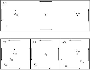
74 |
michael baer |
Figure 3. The breaking up of a region s, which contains two conical intersections (at C12 and C23), into three subregions: (a) The full region s defined in terms of the closed contour . (b) The region s12, which contains a conical intersection at C12 and is defined by the closed contour 12. (c) The region s0, which is defined by the closed contour 0 and does not contain any conical intersection. (d) The region s23, which contains a conical intersection at C23 and is defined by the closed contour 23. It can be seen that ¼ 12 þ 0 þ 23.
If a contour in a given plane surrounds two conical intersections belonging to two different (adjacent) pairs of states, only two eigenfunctions flip sign—the one that belongs to the lowest state and the one that belongs to the highest one.
To prove this, we consider the following three regions (see Fig. 3): In the first region, designated s12, is located the main portion of the interaction, t12, between states 1 and 2 with the point of the conical intersection at C12. In the second region, designated as s23, is located the main portion of the interaction, t23, between states 2 and 3 with the point of the conical intersection at C23. In addition, we assume a third region, s0, which is located in-between the two and is used as a buffer zone. Next, it is assumed that the intensity of the interactions due to the components of t23 in s12 and due to t12 in s23 is 0. This situation can always be achieved by shrinking s12ðs23Þ toward its corresponding center C12ðC23Þ. In s0, the components of both t12 and t23 may be of arbitrary magnitude but no conical intersection of any pair of states is allowed to be there.
76 |
michael baer |
The three equalities can be fulfilled if and only if the two G matrices, namely, G12 and G23, are chosen to be
G12 ¼ D23A0 and G23 ¼ D12A0 |
ð103Þ |
Since the D matrices are diagonal the same applies to D12 and D23 so that D becomes
D ¼ D13 ¼ D12D23 |
ð104Þ |
Our next task will be to obtain D12 and D23. For this purpose, we consider s12 and s23—the two partial s matrices—defined as follows:
s12ðsÞ ¼ |
0 |
0 |
t12 |
0 |
1 |
|
s23ðsÞ ¼ |
0 |
0 |
0 |
0 |
1 |
ð105Þ |
t12 |
0 |
0 |
and |
0 |
0 |
t23 |
|||||||
|
@ |
0 |
0 |
0 A |
|
|
@ |
0 |
t23 |
0 |
A |
|
|
so that |
|
s ¼ s12 þ s23 |
ð106aÞ |
We start with the first of Eqs. (101), namely, |
|
A ¼ G12 ‘ð ij ds s12A |
ð107Þ |
where s12 replaces s because s23 is assumed to be negligibly small in s12. The solution and the corresponding D matrix, namely, D12 are well known (see discussion in Sections V.A.1 and V.B). Thus
01
D12 |
1 |
0 |
0 |
ð |
|
Þ |
¼ @ 0 |
0 |
1 A |
108 |
|||
|
0 |
1 |
0 |
|
|
which implies (as already explained in Section IV.A) that the first (lowest) and the second functions flip sign. In the same way, it can be shown that D23 is equal to
|
@ |
1 |
0 |
0 |
|
|
D23 ¼ |
0 |
0 |
1 A |
ð109Þ |
||
0 |
0 |
1 |
0 |
1 |
||
the electronic non-adiabatic coupling term |
77 |
which shows that the second and the third (the highest) eigenfunctions flip sign. Substituting Eqs. (108) and (109) in Eq. (104) yields the following result for D13:
01
D13 ¼ @ |
1 |
0 |
0 |
ð110Þ |
0 |
1 |
0 |
||
0 |
0 |
1 A |
In other words, surrounding the two conical intersections indeed leads to the flip of sign of the first and the third eigenfunctions, as was claimed.
This idea can be extended, in a straightforward way, to various situations as will be done in Section IX.
IX. THE GEOMETRICAL INTERPRETATION FOR SIGN FLIPS
In Sections V and VII, we discussed the possible K values of the D matrix and made the connection with the number of signs flip based on the analysis given in Section IV.A. Here, we intend to present a geometrical approach in order to gain more insight into the phenomenon of signs flip in the M-state system (M > 2).
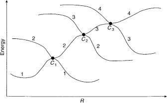
As was already mentioned, conical intersections can take place only between two adjacent states (see Fig. 4). Next, we make the following definitions:
1.Having two consecutive states j and (j þ 1), the two form the conical intersection to be designated as Cj as shown in Figure 4, where NJ conical intersection are presented.
Figure 4. Four interacting adiabatic surfaces presented in terms of four adiabatic curves. The points Cj; j ¼ 1,2,3, stand for the three conical intersections.
78 |
michael baer |
2.The contour that surrounds a conical intersection at Cj will be designated as jjþ1 [see Fig. 5(a)].
3.A contour that surrounds two consecutive conical intersections that is, Cj and Cjþ1 will be designated as jjþ2 [see Fig. 5(b)]. In the same way a contour that surrounds n consecutive conical intersections namely Cj; Cjþ1 . . . Cjþn will be designated as jjþn [see Fig. 5(c) for NJ ¼ 3].
4.In case of three conical intersections or more, a contour that surrounds Cj and Ck but not the in-between conical intersections will be designated asj;k. Thus, for example, 1;3 surrounds C1 and C3 but not C2 (see Fig. 5d).
We also introduce an algebra of closed contours based on the analysis given in Section VIII (see also Appendix C):
Xn 1
jn ¼ |
kkþ1 |
|
ð111Þ |
|
k¼j |
|
|
and also |
|
|
|
j;k ¼ jjþ1 þ kkþ1 |
where |
ðk > j þ 1Þ |
ð112Þ |
This algebra implies that in case of Eq. (111) the only two functions (out of n) that flip sign are z1 and zn because all in-between z functions get their sign flipped twice. In the same way, Eq. (112) implies that all four electronic functions mentioned in the expression, namely, the jth and the (j þ 1)th, the kth and the (k þ 1)th, all flip sign. In what follows, we give a more detailed explanation based on the mathematical analysis of the Section VIII.
In Sections VII and VIII, it was mentioned that K yields the number of eigenfunctions that flip sign when the electronic manifold traces certain closed paths. In what follows, we shall show how this number is formed for various NJ values.
The situation is obvious for NJ ¼ 1. Here, the path either surrounds or does not surround a C1. In case it surrounds it, two functions, that is, z1 and z2, flip sign so that K ¼ 2 and if it does not surround it no z function flips sign and K ¼ 0. In case of NJ ¼ 2, we encounter two conical intersections, namely, C1 and the C2 (see Fig. 5a and 5b). Moving the electronic manifold along the path12 will change the signs of z1 and z2, whereas moving it along the path 23 will change the signs z2 and z3. Next, moving the electronic manifold along the path,13 (and Fig. 5b) causes the sign of z2 to be flipped twice (once when surrounding C1 and once when surrounding C2) and therefore, altogether, its sign remains unchanged. Thus in the case of NJ ¼ 2 we can have either no change of sign (when the path does not surround any conical intersection) or three cases where two different functions change sign.
the electronic non-adiabatic coupling term |
79 |
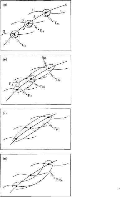
Figure 5. The four interacting surfaces, the three points of conical intersection and the various contours leading to sign conversions: (a) The contours jjþ1 surrounding the respective Cj; j ¼ 1; 2; 3 leading to the sign conversions of the jth and the ( j þ 1)th eigenfunctions. (b) The contours jjþ2 surrounding the two (respective) conical intersections namely Cj and Cjþ1; j ¼ 1; 2 leading to the sign conversions of the jth and the ( j þ 2)th eigenfunctions but leaving unchanged the sign of the middle, the ( j þ 1), eigenfunction. Also shown are the contours jjþ1 surrounding the respective Cj; j ¼ 1; 2; 3 using partly dotted lines. It can be seen thatjjþ2 ¼ jjþ1 þ jþ1jþ2. (c) The contour14 surrounding the three conical intersections, leading to the sign conversions of the first and the fourth eigenfunctions but leaving unchanged the signs of the second and the third eigenfunctions. Based on Figure (5b) we have 14 ¼ 12 þ 23 þ34: (d) The contour 1;3 surrounding the two external conical intersections but not the middle one, leading to the sign conversions of all four eigenfunctions, that is,
ðz1; z2; z3; z4Þ; ! ð z1; z2; z3; z4Þ. Based on Figure (5b) we have 1;3 ¼
12 þ 34.
80 |
michael baer |
A somewhat different situation is encountered in case of NJ ¼ 3, and therefore we shall briefly discuss it as well (see Fig. 5d). It is now obvious that contours of the type jjþ1; j ¼ 1; 2; 3 surround the relevant Cj (see Fig. 5a) and will flip the signs of the two corresponding eigenfunctions. From Eq. (111), we get that surrounding two consecutive conical intersections, namely, Cj and Cjþ1, with jjþ2; j ¼ 1; 2 (see Fig. 5b), will flip the signs of the two external eigenfunctions, namely, zj and zjþ2, but leave the sign of zjþ1 unchanged. We have two such cases—the first and the second conical intersections and the second and the third ones. Then we have a contour 14 that surrounds all three conical intersections (see Fig. 5c) and here, like in the previous where NJ ¼ 2 [see also Eq. (111)], only the two external functions, namely, z1 and z4 flip sign but the two internal ones, namely, z2 and z3, will be left unchanged. Finally, we have the case where the contour 1;3 surrounds C1 and C3 but not C2 (see Fig. 5d). In this case, all four functions flip sign [see Eq. (112)].
We briefly summarize what we found in this NJ ¼ 3 case: We revealed six different contours that led to the sign flip of six (different) pairs of functions and one contour that leads to a sign flip of all four functions. The analysis of Eq. (87) shows that indeed we should have seven different cases of sign flip and one case without sign flip (not surrounding any conical intersection).
X.THE MULTIDEGENERATE CASE
The emphasis in our previous studies was on isolated two-state conical intersections. Here, we would like to refer to cases where at a given point three (or more) states become degenerate. This can happen, for example, when two (line) seams cross each other at a point so that at this point we have three surfaces crossing each other. The question is: How do we incorporate this situation into our theoretical framework?
To start, we restrict our treatment to a tri-state degeneracy (the generalization is straightforward) and consider the following situation:
1.The two lowest states form a conical intersection, presented in terms of t12ðrÞ, located at the origin, namely, at r ¼ 0.
2.The second and the third states form a conical intersection, presented in terms of s23ðr; j j r0; j0Þ, located at r ¼ r0, j ¼ j0 [24].
3.The tri-state degeneracy is formed by letting r0 ! 0, namely,
rlim0 0 s23ðr; j j r0; j0Þ ¼ s23ðr; jÞ |
ð113Þ |
! |
|
so that the two conical intersections coincide. Since the two conical intersections are located at the same point, every closed contour that surrounds one of them will surround the other so that this situation is the case of one contour ð¼ 13Þ
the electronic non-adiabatic coupling term |
81 |
surrounding two conical intersections (see Fig. 5b). According to the discussion of Section IX, only two functions will flip signs (i.e., the lowest and the highest one). Extending this case to an intersection point of n surfaces will not change the final result, namely, only two functions will flip signs, the lowest one and the highest one.
This conclusion contradicts the findings discussed in Sections V.A.2 and V.A.3. In Section V.A.2, we treated a three-state model and found that functions can never flip signs. In Section V.A.3, we treated a four-state case and found that either all four functions flip their sign or none of them flip their sign. The situation where two functions flip signs is not allowed under any conditions.
Although the models mentioned here are of a very specialized form (the nonadiabatic coupling terms have identical spatial dependence), still the fact that such contradictory results are obtained for the two situations could hint to the possibility that in the transition process from the nondegenerate to the degenerate situation, in Eq. (113), something is not continuous.
To date, this contradiction has not been resolved but we still would like to make the following suggestion. In molecular physics, we may encounter two types of multidegeneracy situations: (1) The one described above is formed from an aggregation of two-state conical intersections and depends on external coordinates (the coordinates that form the seam). Thus this multidegeneracy is created by varying these external coordinates in a proper way. In the same way, the multidegeneracy can be removed by varying these coordinates. Note that this kind of a degeneracy is not an essential degeneracy because the main features of the individual conical intersections are unaffected while assembling or disassembling this degeneracy. We shall term this degeneracy as a breakable multidegeneracy. (2) The other type mentioned above is the one that is not formed from an aggregation of conical intersections and therefore will not breakup under any circumstances. Therefore, this degeneracy is termed the unbreakable multidegeneracy.
XI. THE NECESSARY CONDITIONS FOR A RIGOROUS MINIMAL DIABATIC POTENTIAL MATRIX
This Section considers one of the more important dilemmas in molecular physics: Given a Born–Oppenheimer–Huang system, what is the minimal subHilbert space for which diabatization is still valid.
A.Introductory Comments
When studying molecular systems one encounters two almost insurmountable difficulties: (1) That of numerically treating the non-adiabatic coupling terms that are not only spiky—a feature that is in itself a ‘‘recipe’’ for numerical
82 |
michael baer |
instabilities—but also, singular. (2) That of having to consider large portions of the Hilbert space. As we will show in this section, the two apparently unrelated difficulties are strongly interrelated. Moreover, we will show that resolving the first difficulty may, in many cases, also settle the second.
As discussed earlier, one distinguishes between (1) the adiabatic framework that is characterized by the adiabatic surfaces and the non-adiabatic (derivative) coupling terms and (2) the diabatic framework that is characterized by the fact that derivative couplings are eliminated and replaced by (smoothly behaving) potential couplings. Because of the unpleasant features of the non-adiabatic coupling terms the dynamics is expected to be more easily carried out within the diabatic framework. Therefore, transforming to the diabatic framework (also to be termed diabatization) is the right thing to do when treating the multistate problem as created by the Born–Oppenheimer–Huang approach [1,2]. However, because the non-adiabatic coupling terms are frequently singular functions may cause difficulties and therefore the diabatization becomes more of a theoretical– mathematical problem rather than a numerical one.
In 1975, Baer suggested that the diabatic arrangement be reached by first forming the adiabatic framework and then transforming it to the diabatic one by employing the non-adiabatic coupling terms [34]. This approach becomes particularly simple when applied to two states, because it amounts to the calculation of an angle (related to a 2 2 orthogonal matrix), which is formed by integration over the (1,2) non-adiabatic coupling term along a given contour [34–36]. This approach was successfully employed to treat charge-transfer processes [54,94–97], which until that time were solely carried out using classical trajectories [3,98,99], reactive exchange processes between neutrals [100–102] and photodissociation processes [103,104].
Because of difficulties in calculating the non-adiabatic coupling terms, this method did not become very popular. Nevertheless, this approach, was employed extensively in particular to simulate spectroscopic measurements, with a ‘‘modification’’ introduced by Macias and Riera [47,48]. They suggested looking for a symmetric operator that behaves ‘‘violently’’ at the vicinity of the conical intersection and use it, instead of the non-adiabatic coupling term, as the integrand to calculate the adiabatic-to-diabatic transformation. Consequently, a series of operators such as the electronic dipole moment operator, the transition dipole moment operator, the quadrupole moment operator, and so on, were employed for this purpose [49,52,53,105]. However, it has to be emphasized that immaterial to the success of this approach, it is still an ad hoc procedure.
For example, there are also other approaches by Pacher et al. [106], Romero et al. [107], Sidis [40], and Domcke and Stock [42], which developed recipes for construction ab initio diabatic states. These methods can be efficient as long as one encounters, at most, one isolated conical intersection in a given region in