Chau Chemometrics From Basics to Wavelet Transform

5.Perform forward WT to obtain the wavelet coefficients.

6.Display Figure 5.25.

7.Set approximation coefficients with zeros, and construct the signal by applying inverse WT.

8.Display Figure 5.24

Method B:

1.Load experimental spectrum (Fig. 5.24a).

2.Extend the spectral data for avoiding the edge effect.

3.Make a wavelet filter---Daubechies4.

4.Set resolution level J = 5.

5.Perform forward WT to obtain the c and d components with the improved algorithm.

6.Display Figure 5.26.

7.Subtract c4 from the experimental spectrum.

8.Convert the subtracted result to k space.

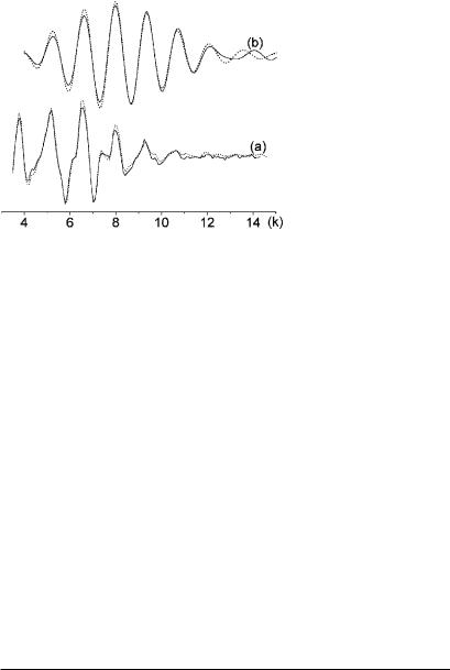
9.Display Figure 5.27, curve (a).

As mentioned above, the aim of analyzing the EXAFS spectrum is to obtain the structural parameters such as N and r in Equation (5.47). In order to obtain the structural parameters from the EXAFS oscillation, Fourier filtering and least-square fitting can be performed. Figure 5.27, curve (b) shows the filtered results for the first coordination shell from the EXAFS signals in Figure 5.27, curve (a), and Table 5.3 compares the structural parameters obtained by least-square fitting of three Cu samples. The last column in the table shows a comparison of the fitted errors, which is

Figure 5.26. Plots of the approximations obtained by applying WT to the experimental EXAFS spectrum with the improved algorithm.

Figure 5.27. Background-removed results by conventional (solid line) and WT (dotted line) methods (a), and their filtered results (b).

calculated by

where N is the number of points in the spectra and Xcali and Xexpi are, respectively, the fitted and the experimental values. For the sake of com-

parison between the two methods, both of the experimental and the fitted spectra were normalized when calculating the fitted error.

From Figure 5.27, curve (b), it is clear that the result by WT method is superior to that of the cubic spline method. From Table 5.3 it can be seen that, except for the coordination distance r , which is very close to the results of the two methods, all the other three parameters obtained by the wavelet transform method are larger than the results of cubic spline method. But they are reasonable. The fitted errors are also improved by the WT method. Table 5.3 also shows that the reproducibility of the three results

Table 5.3. Comparison of Structural Parameters and Fitted Errors Obtained by Least-Squares-Fitting from Background-Removed Spectra with WT and Spline Method Respectively

obtained by wavelet transform method is obviously superior to that of the cubic spline method. The reason for this is that the cubic spline method performs the background removal according to the points selected by the operator. However, there is no operator interference in the WT method.

5.3.3. Baseline Correction

Baseline drift is caused mainly by continuous variations of experiment conditions, such as temperature, solvent programming in liquid chromatography, or temperature programming in gas chromatography. Therefore, baseline drift is a very common problem in chromatographic studies.

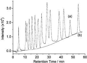
Figure 5.28 shows an example of the separation of the drifting baseline from a chromatogram with gradient elution by method B. Curve (a) is the experimental chromatogram. From the figure, it can be seen that there is a strong baseline drift caused by the gradient elution in the chromatogram. Curve (b) is the 8th-scale discrete approximation c8 decomposed by WT with Symmlet (S5) wavelet. Apparently, it resembles the baseline. Figure 5.29 shows the result obtained by subtracting curve (b) from curve (a) of Figure 5.28 with a factor f of 0.93. From the result, it is clear that the removal of baseline by this method is complete and satisfactory.

5.3.4. Background Removal Using Continuous

Wavelet Transform

As stated in Chapter 4, the CWT of a signal s(t ) with an analyzing wavelet ψ(t ) is the convolution of s(t ) with a scaled and conjugated wavelet

Figure 5.28. An experimental chromatogram (a) and its eighth discrete approximation obtained by WT decomposition (b).

the each component are close to each other, we cannot obtain satisfactory results using this equation because

the second term in the equation is a sum over the other spectral lines, with the amplitudes attenuated by the exponential factor.

Therefore, in practical applications, we can define

and iterate the procedure with sl(k −1)(b) as the new input signal. After a certain number of iterations, the second term in Equation (5.59) will become negligible.

Example 5.9: Large Spectral Line Removal of a Simulated NMR Spectrum. The NMR signal in Fourier domain can be simulated by

Figure 5.30 shows three simulated signals s1(t ), s2(t ), and s(t ) = s1(t ) + s2(t ) and their Fourier transforms, where s1(t ) and s2(t ) were simulated by

where t is sampled by 2048 data points. It can be seen that the large spectral line s1(t ) can be viewed as the baseline or the background of the small peak s2(t ).

In order to separate the signals s1(t ) and s2(t ) from the mixed signal, we can use the iterative procedure described by Equation (5.60). Figure 5.31 shows the results at the number of the iteration k = 100, 200, and 300. In the calculation, Morlet wavelet, which is defined by

and σ0 = 1, ω0 = 5 were adopted. Because the aim is to remove the s1(t ) and extract s2(t ), al = ω0/ω1 = 5/0.2π was used. It can be seen that, after 500 iterations, the large spectral line is completely removed.

sampling points. The data matrix can be divided into two parts:

Here Xc originated from chemical components and Xb from noise and background. For the sake of convenience, we assume that the data matrix is free of noise; Xb will composed of spectral and chromatographic background. The background of 2D analytical data matrices such as the ‘‘hyphenated’’ chromatographic--spectroscopic data generally has the following properties: (1) there is no direct correlation between the chromatographic baseline drift and the spectral background, (2) there is a very similar spectral background at the two ends of a chromatographic peak, and (3) there is a similar drift of the baseline at each retention time since the scanning time for each spectrum is very short. Thus, the background matrix can be written as

where t denotes the baseline drift in chromatographic direction, sT denotes the spectral background, and 1 and 1T denote that a vector contains only 1s. The superscript T denotes transposition.

Therefore, the spectrum at retention time i can be expressed as

where xcT,i denotes a ‘‘pure’’ spectrum at retention time i and ti corresponding to the baseline drift at the retention time. In a zero-component regions, xcT,i should be a zero vector. Equation (5.68) turns into

Equation (5.69) shows that the spectra in zero-component regions before and after elution should be similar if there is spectral background. If not, they should be flat lines. Therefore, the zero component regions may be used to detect the presence of spectral background.

According to the algorithm of WT, we can obtain approximation and detail coefficients by using Equations (5.3) and (5.4). The detail coefficients of a spectrum at retention time i on scale k can be expressed as

According to the properties of the filters H and G, it is easy to deduce that the detail coefficients of a constant vector c = {c, c, . . . , c} should be

In zero-component regions, this last equation can be further reduced into

Therefore, using Equations (5.72) and (5.73), we can remove both the chromatographic baseline drift and the spectral background.

For example, Figure 5.33a,b shows two simulated chromatographic peaks and two simulated spectra, which are used to simulate a theoretical HPLC-DAD data matrix (denoted as X). Figure 5.33c,d shows a simulated chromatographic baseline and a simulated spectral background, which are used to simulate an HPLC-DAD data matrix containing baseline drift and background. We can simulate two data matrices X1 and X2,

Figure 5.33. Chromatograms (a), spectra (b), chromatographic baseline (c), and spectral background (d) used in the simulation of the HPLC-DAD data matrices.