126 6 Scheduling and Resource Binding

The initial word-length compatibility graph is constructed in the following manner: A resource set R is constructed following (6.5–6.8). Edge set H is initialized to the set {{v V, r R} : r R(v)}. C is initialized to the empty set. As Algorithm ArchSynth executes, word-length refinement will result in the deletion of edges from the set H.

6.4.3 Resource Bounds

The first stage of the heuristic is to find the smallest and largest sensible upper bounds to place on the number of multipliers required. These values are obtained from a study of how the iteration latency achieved by list-scheduling decreases with the number of multipliers allowed.

A standard resource-constrained list scheduling algorithm [DeM94, NT86] can be used to heuristically obtain these bounds. Standard ALAP urgencybased list scheduling with a bound c N2 on the number of resources of each type is used. c is a 2-vector of integer elements, the first corresponding to the bound on the number of multipliers and the second corresponding to the bound on the number of adders.

The bounds mmin and mmax used in Algorithm ArchSynth can now be defined, assuming that the given latency bound is realizable. Bound mmin is the smallest value such that the list-scheduled latency is within the constraint

for all schedules with c ≥ (mmin, βmmin) and (v) = min(v) for all v V . Similarly bound mmax is the smallest value such that the list-scheduled

latency is within the constraint for all schedules with c ≥ (mmax, βmmax) and (v) = max(v) for all v V . For tight latency constraints there may be no such mmax value, in which case mmax is set to |Vm|. In each of these cases, a binary search is used to determine the bounds.

The rationale behind these bounds is the following. If an algorithm cannot be scheduled to meet the imposed latency constraint under a resource constraint c, even when all operations have their minimum possible latency, then the algorithm cannot meet this latency constraint for any c ≤ c. This provides a lower bound on the number of each type of resource required. Similarly, if the imposed timing constraint can be met under a resource constraint c, even when all operations have their maximum latency, then the algorithm can meet this latency constraint for all c ≥ c. This provides an upper bound on the number of each type of resource required. Fig. 6.5 illustrates the way in which the achieved latency varies with the bound on the number of multipliers supplied to the list-scheduler.

Example 6.8. An example derivation of resource bounds is illustrated in Fig. 6.6. Fig. 6.6(a) illustrates a simple data flow graph, with corresponding initial word-length compatibility graph shown in Fig. 6.6(b). The latency curves resulting from list scheduling for di erent resource bounds are plotted in Fig. 6.6(c). The points corresponding to the minimum possible number and maximum necessary number of multiplier resources have been highlighted.

end

Using Algorithm LatencyBounds, an upper bound on the latency of each operation can be established. Once this has been done, the set of edges H of the Word-Length Compatibility Graph, representing the possible design decisions, has been pruned.

6.4.5 Scheduling with Incomplete Word-Length Information

At the time of scheduling in Algorithm ArchSynth, the word-length of each operation may not be fixed. Indeed each operation could be implemented using any resource type to which the operation is linked by an edge in the word-length compatibility graph. The scheduling problem therefore has incompletely defined constraints [CSH00], and a technique must be developed to incorporate these constraints into directing the search for a solution. The following paragraphs illustrate the need for such a technique, before introducing the proposed solution.

Traditional resource-constrained scheduling techniques such as force-directed list scheduling [PK89], require resource constraints to be expressed in terms of a bound on the number of resources of each type. During standard list scheduling, these constraints are tested at each time step before deciding whether to schedule a new operation. The constraints may be formally expressed as follows. Let ev,t be defined as in (6.24). Thus ev,t = 1 i operation v is executing during time-step t. Given a set of control steps T (6.15), a set of operations V , and the maximum number of resources ck of type k, the traditional resource constraints may be expressed as (6.25).

In the case of multiple word-length systems, these constraints tend to be too relaxed to guarantee that no more than ak resources of type k will be used by the given schedule.

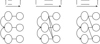
Example 6.9. Consider the schedules and corresponding word-length compatibility graphs shown in Fig. 6.7. Such graphs could arise during the execution of Algorithm ArchSynth. Fig. 6.7(a) has fully defined word-length information for each operation. It is clear that even though v1, v2 and v3 are all multiplications and do not overlap in execution, three distinct multiplier resources will still be required for their implementation. However the standard scheduling constraint (6.25) would be satisfiable for amult = 1.

Fig. 6.7(b) has an incomplete specification (there is at least one operation which could be implemented in more than one possible resource type). However a 32 × 32-bit multiplier could conceivably implement every operation.

Fig. 6.7. Some schedules and word-length compatibility graphs

Thus it is possible to implement the entire system using a single multiplier resource.

Fig. 6.7(c) illustrates a general case, corresponding to the deletion of a single edge from the word-length compatibility graph of Fig. 6.7(b). Using traditional methods, it is unclear in this case how to incorporate such constraints into the search for an appropriate schedule.

These examples demonstrate that a more sophisticated approach to scheduling is required to take word-length information into account. In general it is necessary to consider the incomplete word-length specification provided by an edge set H.

The scheduling algorithm proposed is a modification of standard list scheduling [DeM94]. The modification lies in the resource constraint calculation. Before any scheduling takes place, a small cardinality subset S R is found such that v V, s S : {v, s} H. Conceivably, a resource binding could consist only of resource of types represented in S. Define

S(v) = {s S : {v, s} H}. Then the proposed constraint function to be used in the algorithm can be expressed as in (6.26).

k {add, mult},

This is a heuristic measure with the following justification. Firstly (6.26) is at least as strict as (6.25), which is a special case of the former under the condition |type(V )| = |S|, the smallest sized S possible. This represents the

case where each multiplication could be performed by a single large multiplier, and each addition could be performed by a single large adder. As the possibilities for the implementation of each operation are reduced during execution of Algorithm ArchSynth, the balance on the left hand side of (6.26)

cardinality S is used in order to relax the constraint as much as possible, since any two operations in O(s) could possibly be eventually bound to the same resource. Operations belonging to more than one O(s), i.e. those v V with |S(v)| > 1, are accounted for by ‘sharing’ equally their usage between each of the elements S(v).

Algorithm IncompSched illustrates this scheduling based on incomplete information. Two auxilliary data structures are used in the algorithm to keep track of the scheduling constraint (6.26), usage(s) and maxusage(s). Respectively, these keep track of the instantaneous and peak usage of resource type s S. The algorithm starts by setting the latency (v) of each operation to its maximum (step 1). After so doing, a standard ALAP-based urgency measure [DeM94] is calculated for each node (step 2), and the time step index is initialized (step 3). The set S described above (step 4), and its related function S(v) (step 5), to be used in the scheduling constraint (6.26) are then calculated. Step 6 ensures that the peak usage maxusage(s) for each element of that set is initialized. The algorithm then enters its main scheduling loop, with one iteration per time step (step 7).

At the start of each iteration, the instantaneous usage of resources is initialized (step 7.1), the ready-list is calculated (step 7.2), and the prime candidate for scheduling is selected (step 7.3). The algorithm then enters a secondary loop (step 7.4), which tries to schedule this and any other operation of the same type. The current left-hand side of (6.26) is first calculated (step 7.4.1), and then updated (step 7.4.2) for any s S for which scheduling in the current control step would use more than the current peak usage for that s. If the updated (6.26) is still satisfied, then the scheduling of the operation is accepted (step 7.4.3), and the peak usage is updated (step 7.4.4). Deadlocks, to be discussed below, may occur in the scheduling process. These are detected by step 7.5.

Example 6.10. An example execution of Algorithm IncompSched is shown in Fig. 6.8. The data flow graph and word-length compatibility graph are shown in Figs. 6.8(a) and (b) respectively. Fig. 6.8(c) enumerates the S(v) sets for this example, and Fig. 6.8(d) shows how the usage and maxusage variables

evolve as the algorithm executes for aadd = 1, amult = 2. The resulting schedule is shown in Fig. 6.8(e), and could be resource-bound as a single

16-bit adder together with both a 16 × 16-bit multiplier and a 32 × 32-bit multiplier. Details on how such a resource binding can be found for general graphs are discussed in the following section.

5.Let S(v) = {s S : {v, s} H}

6.maxusage(s) ← 0 for all s S

7.do

7.1usage(s) ← 0 for all s S

7.2E ← the list-schedule ‘ready list’ [DeM94], sorted by urgency

7.3e ← most urgent element of E

7.4do

7.4.1 total ← maxusage(s)

s S({v V :type(v)=type(e)})

7.4.2foreach s S(e):

usage(s) + |S(e)|−1 > maxusage(s) do total ← total − maxusage(s)+

usage(s) + |S(e)|−1 end foreach

7.4.3 if total ≤ atype(e) do

S(e) ← t

usage(s) ← usage(s) + |S(e)|−1

7.4.4foreach s S(e) : usage(s) > maxusage(s) do

maxusage(s) ← usage(s) end foreach

end if

7.4.5 e ← next most urgent element of E, if one exists while such an e exists k {add, mult} :

maxusage(s) < ai

s S:type(s)=k

t ← t + 1

7.5 if deadlock detected do return failure case

end if

while there remains at least one unscheduled operation

end

There are a number of significant di erences between standard list scheduling and Algorithm IncompSched. Information on resource usage is accumulated over control steps in Algorithm IncompSched, rather than each step being constraint-function-independent of each other step. There are two related drawbacks from this: Firstly, it is possible for the proposed list-scheduler to deadlock, by scheduling operations belonging to O(s1) for the some s1 S early in the schedule and then having no remaining resources to schedule operations belonging to O(s2) for some s2 S, s2 =s1 later in the schedule. Such deadlocks can be easily detected: if all operations have finished by the current time-step and yet no operation has been scheduled by the end of that time-step, deadlock has occurred. Secondly, although the scheduler may not deadlock, greedy allocation of parallel O(s1) operations early-on in the schedule may cause schedules of longer than optimal latency. Thus Algorithm IncompSched has a greedy bias towards earlier time steps.