

Brereton Chemometrics
.pdfEXPERIMENTAL DESIGN |
49 |
|
|
•The value is always greater than 0.
•The lower the value, the higher is the confidence in the prediction. A value of 1 indicates very poor prediction. A value of 0 indicates perfect prediction and will not be achieved.
•If there are P coefficients in the model, the sum of the values for leverage at each experimental point adds up to P . Hence the sum of the values of leverage for the 12 experiments in Table 2.14 is equal to 6.
In the design in Table 2.14, the leverage is lowest at the centre, as expected. However, the value of leverage for the first four points in slightly lower than that for the second four points. As discussed in Section 2.4, this design is a form of central composite design, with the points 1–4 corresponding to a factorial design and points 5–8 to a star design. Because the leverage, or confidence, in the model differs, the design is said to be nonrotatable, which means that the confidence is not solely a function of distance from the centre of experimentation. How to determine rotatability of designs is discussed in Section 2.4.3.
Leverage can also be converted to equation form simply by substituting the algebraic expression for the coefficients in the equation
h = d.(D .D)−1.d
where, in the case of Table 2.14,
d = ( 1 x1 x2 x12 x22 x1x2 )
to give an equation, in this example, of the form
h = 0.248 − 0.116(x12 + x22) + 0.132(x14 + x24) + 0.316x12x22
The equation can be obtained by summing the appropriate terms in the matrix (D .D)−1. This is illustrated graphically in Figure 2.16. Label each row and column by the corresponding terms in the model, and then find the combinations of terms in the matrix
|
|
1 |
x1 |
|
x2 |
|
x12 |
x22 |
x1x2 |
|
|
|
|
|
|
|
|
|
|
|
|
1 |
|
0.248 |
|
0 |
|
0 |
−0.116 |
−0.116 |
0 |
|
|
|
|
|
|||||||
|
|
|
|
|
|
|
|
|
|
|
x1 |
0 |
|
0.118 |
|
0 |
0 |
0 |
0 |
||
|
|
|
|
|||||||
x2 |
0 |
|
0 |
|
0.118 |
0 |
0 |
0 |
||
|
|
|
|
|||||||
|
|
|
|
|
|
|
|
|
|
|
x |
2 |
|
|
|
|
|
|
|
|
|
|
1 |
−0.116 |
|
0 |
|
0 |
0.132 |
0.033 |
0 |
|
|
|
|
|
|||||||
x22 |
−0.116 |
|
0 |
|
0 |
0.033 |
0.132 |
0 |
||
|
|
|||||||||
|
|
|
|
|||||||
x1x2 |
0 |
|
0 |
|
0 |
0 |
0 |
0.25 |
|
|
|
|
|
||||||||
|
|
|
|
|
|
|
|
|
|
|
Figure 2.16
Method of calculating equation for leverage term x12x22

50 |
CHEMOMETRICS |
|
|
that result in the coefficients of the leverage equation, for x12x22 there are three such combinations so that the term 0.316 = 0.250 + 0.033 + 0.033.
This equation can also be visualised graphically and used to predict the confidence of any point, not just where experiments were performed. Leverage can also be used to predict the confidence in the prediction under any conditions, which is given by
y± = s [F(1,N −P )(1 + h)]
√
where s is the root mean square residual error given by Sresid /(N − P ) as determined in Section 2.2.2, the F -statistic as introduced in Section 2.2.4.4, which can be obtained at any desired level of confidence but most usually at 95 % limits and is one-sided. Note that this equation technically refers to the confidence in the individual prediction and there is a slightly different equation for the mean response after replicates have been averaged given by
y± = s F(1,N −P ) |
M + h |
|
|
1 |
|
See Section 2.2.1 for definitions of N and P ; M is the number of replicates taken at a given point, for example if we repeat the experiment at 10 mM five times, M = 5. If repeated only once, then this equation is the same as the first one.
Although the details of these equations may seem esoteric, there are two important considerations:
•the shape of the confidence bands depends entirely on leverage;
•the size depends on experimental error.
These and most other equations developed by statisticians assume that the experimental error is the same over the entire response surface: there is no satisfactory agreement for how to incorporate heteroscedastic errors. Note that there are several different equations in the literature according to the specific aims of the confidence interval calculations, but for brevity we introduce only two which can be generally applied to most situations.
Table 2.15 Leverage for three possible single variable designs using a two parameter linear model.
|
Concentration |
|
|
|
Leverage |
|
|
|
|
|
|
|
|
Design A |
Design B |
Design C |
|
Design A |
Design B |
Design C |
|
|
|
|
|
|
|
1 |
1 |
1 |
0.234 |
0.291 |
0.180 |
|
1 |
1 |
1 |
0.234 |
0.291 |
0.180 |
|
1 |
2 |
1 |
0.234 |
0.141 |
0.180 |
|
2 |
2 |
1 |
0.127 |
0.141 |
0.180 |
|
2 |
3 |
2 |
0.127 |
0.091 |
0.095 |
|
3 |
3 |
2 |
0.091 |
0.091 |
0.095 |
|
4 |
3 |
2 |
0.127 |
0.091 |
0.095 |
|
4 |
4 |
3 |
0.127 |
0.141 |
0.120 |
|
5 |
4 |
3 |
0.234 |
0.141 |
0.120 |
|
5 |
5 |
4 |
0.234 |
0.291 |
0.255 |
|
5 |
5 |
5 |
0.234 |
0.291 |
0.500 |
|
|
|
|
|
|
|
|

EXPERIMENTAL DESIGN |
51 |
|
|
To show how leverage can help, consider the example of univariate calibration; three designs A–C (Table 2.15) will be analysed. Each experiment involves performing 11 experiments at five different concentration levels, the only difference being the arrangement of the replicates. The aim is simply to perform linear calibration to produce a model of the form y = b0 + b1x, where x is the concentration, and to compare how each design predicts confidence. The leverage can be calculated using the design matrix D, which consists of 11 rows (corresponding to each experiment) and two columns (corresponding to each coefficient). The hat matrix consists of 11 rows and 11 columns, the numbers on the diagonal being the values of leverage for each experimental point. The leverage for each experimental point is given in Table 2.15. It is also possible to obtain a graphical representation of the equation as shown in Figure 2.17 for designs A–C.
What does this tell us?
•Design A contains more replicates at the periphery of the experimentation than design B, and so results in a flatter graph. This design will provide predictions that are fairly even throughout the area of interest.
•Design C shows how replication can result in a major change in the shape of the curve for leverage. The asymmetric graph is a result of replication regime. In fact, the best predictions are no longer in the centre of experimentation.
Leverage
0.6
0.4
0.2
0
|
|
|
|
|
|
|
|
|
0.6 |
|
|
|
|
|
|
|
|
|
|
|
|
|
|
|
Leverage |
0.4 |
|
|
|
|
|
|
|
|
|
|
|
|
|
|
|
0.2 |
|
|
|
|
|
|
|
|
|
|
|
|
|
|
|
|
|
|
|
|
|
|
|
|
|
|
|
|
|
|
|
|
|
|
0 |
|
|
|
|
|
|
|
0 |
1 |
2 |
3 |
|
4 |
5 |
6 |
|
|
0 |
1 |
2 |
3 |
4 |
5 |
6 |
|
|
Concentration |
|
|
|
|
|
|
|
|
Concentration |
|
|
|
||
|
|
|
(a) |
|
|
|
|
|
|
|
|
|
(b) |
|
|
|
|
|
|
|
0.6 |
|
|
|
|
|
|
|
|
|
|
|
|
|
|
|
Leverage |
0.4 |
|
|
|
|
|
|
|
|
|
|
|
|
|
|
|
0.2 |
|
|
|
|
|
|
|
|
|
|
|
|
|
|
|
|
|
|
|
|
|
|
|
|
|
|
|
|
|
|
|
|
|
|
0 |
|
|
|
|
|
|
|
|
|
|
|
|
|
|
|
|
0 |
|
1 |
2 |
|
3 |
4 |
5 |
|
6 |
|
|
|
|
|
|
|
|
|
|
Concentration |
|
|
|
|
|
|
|||
|
|
|
|
|
|
|
|
|
(c) |
|
|
|
|
|
|
|
Figure 2.17
Graph of leverage for designs in Table 2.15.

52 |
CHEMOMETRICS |
|
|
 0.4
0.4
(mM)
2 x
0.3
0.5
1
0
0.7 |
0.9 |
x1 mM |
|
Figure 2.18
Two factor design consisting of five experiments
This approach can used for univariate calibration experiments more generally. How many experiments are necessary to produce a given degree of confidence in the prediction? How many replicates are sensible? How good is the prediction outside the region of experimentation? How do different experimental arrangements relate? In order to obtain an absolute value of the confidence of predictions, it is also necessary, of course, to determine the experimental error, but this together, with the leverage, which is a direct consequence of the design and model, is sufficient information. Note that leverage will change if the model changes.
Leverage is most powerful as a tool when several factors are to be studied. There is no general agreement as to the definition of an experimental space under such circumstances. Consider the simple design of Figure 2.18, consisting of five experiments. Where does the experimental boundary stop? The range of concentrations for the first compound is 0.5–0.9 mM and for the second compound 0.2–0.4 mM. Does this mean we can predict the response well when the concentrations of the two compounds are at 0.9 and 0.4 mM, respectively? Probably not, as some people would argue that the experimental region is a circle, not a square. For this nice symmetric arrangement of experiments it is possible to envisage an experimental region, but imagine telling the laboratory worker that if the concentration of the second compound is 0.34 mM then if the concentration of the first is 0.77 mM the experiment is within the region, whereas if it is 0.80 mM it is outside. There will be confusion as to where the model starts and stops. For some supposedly simply designs such as a full factorial design the definition of the experimental region is even harder to conceive.
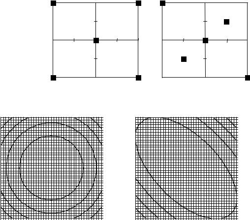
The best solution is to produce a simple graph to show how confidence in the prediction varies over the experimental region. Consider the two designs in Figure 2.19. Using a very simple linear model, of the form y = b1x1 + b2x2, the leverage for both designs is as given Figure 2.20. The consequence of the different experimental arrangements is now obvious, and the result in the second design on the confidence in predictions can be seen. Although a two factor example is fairly straightforward, for multifactor designs
EXPERIMENTAL DESIGN |
53 |
|
|
|
|
|
|
(a) |
|
|
2 |
|
|
(b) |
|
|
|
2 |
|
|
|
|
|
|
|
|
|
|
1 |
|
|
|
|
|
|
1 |
|
|
|
|
|
|
|
−2 |
|
−1 |
0 |
1 |
2 |
|
−2 |
|
−1 |
0 |
|
|
|
|
|
|
|
|
0 |
|
|
|
0 |
1 |
2 |
||||||
|
|
|
|
|
|
|
−1 |
|
|
|
|
|
|
−1 |
|
|
|
|
|
|
|
|
|
|
−2 |
|
|
|
|
|
|
−2 |
|
|
|
|
|
|
Figure 2.19 |
|
|
|
|
|
|
|
|
|
|
|
|
|
|
|
|
|
Two experimental arrangements |
|
|
|
|
|
|
|
|
|
|||||
(a) |
|
|
|
|
|
|
|
2.00 |
(b) |
|
|
|
|
|
|
|
2.00 |
|
|
|
|
|
|
|
|
1.50 |
|
|
|
|
|
|
|
|
1.50 |
|
|
|
|
|
|
|
|
1.00 |
|
|
|
|
|
|
|
|
1.00 |
|
|
|
|
|
|
|
|
0.50 |
|
|
|
|
|
|
|
|
0.50 |
|
|
|
|
|
|
|
|
0.00 |
|
|
|
|
|
|
|
|
0.00 |
|
|
|
|
|
|
|
|
−0.50 |
|
|
|
|
|
|
|
|
−0.50 |
|
|
|
|
|
|
|
|
−1.00 |
|
|
|
|
|
|
|
|
−1.00 |
|
|
|
|
|
|
|
|
−1.50 |
|
|
|
|
|
|
|
|
−1.50 |
|
|
|
|
|
|
|
|
−2.00 |
|
|
|
|
|
|
|
|
−2.00 |
−2.0 |
−1.5 |
−1.0 |
−0.5 |
0.0 |
0.5 |
1.0 |
1.5 |
2.0 |
−2.0 |
−1.5 |
−1.0 |
−5.0 |
0.0 |
0.5 |
1.0 |
1.5 |
2.0 |
Figure 2.20
Graph of leverage for experimental arrangements in Figure 2.19
(e.g. mixtures of several compounds) it is hard to produce an arrangement of samples in which there is symmetric confidence in the results over the experimental domain.
Leverage can show the effect of changing an experimental parameter such as the number of replicates, or, in the case of central composite design, the position of the axial points (see Section 2.4). Some interesting features emerge from this analysis. For example, confidence is not always highest in the centre of experimentation, depending on the number of replicates. The method in this section is an important tool for visualising how changing design relates to the ability to make quantitative predictions.
2.3 Factorial Designs
In this and the remaining sections of this chapter we will introduce a number of possible designs, which can be understood using the building blocks introduced in Section 2.2.

54 |
CHEMOMETRICS |
|
|
Factorial designs are some of the simplest, often used for screening or when there are a large number of possible factors. As will be seen, they have limitations, but are the easiest to understand. Many designs are presented as a set of rules which provide the experimenter with a list of conditions, and below we will present the rules for many of the most common methods.
2.3.1 Full Factorial Designs
Full factorial designs at two levels are mainly used for screening, that is, to determine the influence of a number of effects on a response, and to eliminate those that are not significant, the next stage being to undertake a more detailed study. Sometimes, where detailed predictions are not required, the information from factorial designs is adequate, at least in situations where the aim is fairly qualitative (e.g. to improve the yield of a reaction rather than obtain a highly accurate rate dependence that is then interpreted in fundamental molecular terms).
Consider a chemical reaction, the performance of which is known to depend on pH and temperature, including their interaction. A set of experiments can be proposed to study these two factors, each at two levels, using a two level, two factor experimental design. The number of experiments is given by N = lk , where l is the number of levels (=2), and k the number of factors (=2), so in this case N = 4. For three factors, the number of experiments will equal 8, and so on, provided that the design is performed at two levels only. The following stages are used to construct the design and interpret the results.
1.The first step is to choose a high and low level for each factor, for example, 30◦ and 60◦, and pH 4 and 6.
2.The next step is to use a standard design. The value of each factor is usually coded (see Section 2.2.4.1) as − (low) or + (high). Note that some authors use −1 and +1 or even 1 and 2 for low and high. When reading different texts, do not get confused: always first understand what notation has been employed. There is no universally agreed convention for coding; however, design matrices that are symmetric around 0 are almost always easier to handle computationally. There are four possible unique
sets of experimental conditions which can be represented as a table analogous to four binary numbers, 00 (−−), 01 (−+), 10 (+−) and 11 (++), which relate to a set of physical conditions.
3.Next, perform the experiments and obtain the response. Table 2.16 illustrates the coded and true set of experimental conditions plus the response, which might, for example be the percentage of a by-product, the lower the better. Something immediately appears strange from these results. Although it is obvious that the higher
Table 2.16 Coding of a simple two factor, two level design and the response.
Experiment |
Factor 1 |
Factor 2 |
Temperature |
pH |
Response |
No. |
|
|
|
|
|
|
|
|
|
|
|
1 |
− |
− |
30 |
4 |
12 |
2 |
− |
+ |
30 |
6 |
10 |
3 |
+ |
− |
60 |
4 |
24 |
4 |
+ |
+ |
60 |
6 |
25 |
EXPERIMENTAL DESIGN |
|
|
|
|
|
|
|
55 |
||
|
|
|
|
|
|
|
|
|
|
|
Table 2.17 |
Design matrix. |
|
|
|
|
|
|
|
|
|
|
|
|
|
|
|
|
|
|
|
|
|
Intercept |
Temperature |
pH |
Temp. pH |
|
b0 |
b1 |
b2 |
b12 |
|
1 |
30 |
4 |
120 |
+ |
− |
− |
− |
|||
1 |
30 |
6 |
180 |
+ |
− |
+ |
− |
|||
1 |
60 |
4 |
240 |
−−→+ |
+ |
− |
+ |
|
||
|
1 |
60 |
6 |
360 |
|
+ |
+ |
+ |
+ |
|
the temperature, the higher is the percentage by-product, there does not seem to be any consistent trend as far as pH is concerned. Provided that the experimental results were recorded correctly, this suggests that there must be an interaction between temperature and pH. At a lower temperature, the percentage decreases with increase in pH, but the opposite is observed at a higher temperature. How can we interpret this?
4.The next step, of course, is to analyse the data, by setting up a design matrix (see Section 2.2.3). We know that an interaction term must be taken into account,
and set up a design matrix as given in Table 2.17 based on a model of the form y = b0 + b1x1 + b2x2 + b11x1x2. This can be expressed either as a function of the true or coded concentrations, but, as discussed in Section 2.2.4.1, is probably best as coded values. Note that four possible coefficients that can be obtained from the four experiments. Note also that each of the columns in Table 2.17 is different. This is an important and crucial property and allows each of the four possible terms to be distinguished uniquely from one another, and is called orthogonality. Observe, also, that squared terms are impossible because four experiments can be used to obtain only a maximum of four terms, and also the experiments are performed at only two levels; ways of introducing such terms will be described in Section 2.4.
5.Calculate the coefficients. It is not necessary to employ specialist statistical software for this. In matrix terms, the response can be given by y = D.b, where b is a vector
of the four coefficients and D is presented in Table 2.17. Simply use the matrix inverse so that b = D−1.y. Note that there are no replicates and the model will exactly fit the data. The parameters are listed below.
•For raw values: intercept = 10
temperature coefficient = 0.2 pH coefficient = −2.5 interaction term = 0.05
•For coded values:
intercept = 17.5
temperature coefficient = 6.75 pH coefficient = −0.25 interaction term = 0.75
6.Finally, interpret the coefficients. Note that for the raw values, it appears that pH is much more influential than temperature, and also that the interaction is very small. In addition, the intercept term is not the average of the four readings. The
reason why this happens is that the intercept is the predicted response at pH 0 and 0 ◦C, conditions unlikely to be reached experimentally. The interaction term
appears very small, because units used for temperature correspond to a range of 30 ◦C as opposed to a pH range of 2. A better measure of significance comes from
56 |
CHEMOMETRICS |
|
|
the coded coefficients. The effect of temperature is overwhelming. Changing pH has a very small influence, which is less than the interaction between the two factors, explaining why the response is higher at pH 4 when the reaction is studied at 30 ◦C, but the opposite is true at 60 ◦C.
Two level full factorial designs (also sometimes called saturated factorial designs), as presented in this section, take into account all linear terms, and all possible k way interactions. The number of different types of terms can be predicted by the binomial theorem [given by k!/(k − m)!m! for mth-order interactions and k factors, e.g. there are six two factor (=m) interactions for four factors (=k)]. Hence for a four factor, two level design, there will be 16 experiments, the response being described by an equation with a total of 16 terms, of which
•there is one interaction term;
•four linear terms such as b1;
•six two factor interaction terms such as b1b2;
•four three factor interactions terms such as b1b2b3;
•and one four factor interaction term b1b2b3b4.
The coded experimental conditions are given in Table 2.18(a) and the corresponding design matrix in Table 2.18(b). In common with the generally accepted conventions, a + symbol is employed for a high level and a − for a low level. The values of the interactions are obtained simply by multiplying the levels of the individual factors together. For example, the value of x1x2x4 for the second experiment is + as it is a product of − × − × +. Several important features should be noted.
•Every column (apart from the intercept) contains exactly eight high and eight low levels. This property is called balance.
•Apart from the first column, each of the other possible pairs of columns have the property that each for each experiment at level + for one column, there are equal number of experiments for the other columns at levels + and −. Figure 2.21 shows a graph of the level of any one column (apart from the first) plotted against the level of any other column. For any combination of columns 2–16, this graph will be identical, and is a key feature of the design. It relates to the concept of orthogonality, which is used in other contexts throughout this book. Some chemometricians regard each column as a vector in space, so that any two vectors are at right angles to each other. Algebraically, the correlation coefficient between each pair of columns equals 0. Why is this so important? Consider a case in which the values of two factors (or indeed any two columns) are related as in Table 2.19. In this case, every time the first factor is at a high level, the second is at a low level and vice versa.
Thus, for example, every time a reaction is performed at pH 4, it is also performed at 60 ◦C, and every time it is performed at pH 6, it is also performed at 30 ◦C, so how can an effect due to increase in temperature be distinguished from an effect due to decrease in pH? It is impossible. The two factors are correlated. The only way to be completely sure that the influence of each effect is independent is to ensure that the columns are orthogonal, that is, not correlated.
•The other remarkable property is that the inverse of the design matrix is related to the transpose by
D−1 = (1/N )D

EXPERIMENTAL DESIGN |
57 |
|
|
Table 2.18 Four factor, two level full factorial design.
(a) Coded experimental conditions
Experiment No. |
Factor 1 |
Factor 2 |
Factor 3 |
Factor 4 |
|
|
|
|
|
1 |
− |
− |
− |
− |
2 |
− |
− |
− |
+ |
3 |
− |
− |
+ |
− |
4 |
− |
− |
+ |
+ |
5 |
− |
+ |
− |
− |
6 |
− |
+ |
− |
+ |
7 |
− |
+ |
+ |
− |
8 |
− |
+ |
+ |
+ |
9 |
+ |
− |
− |
− |
10 |
+ |
− |
− |
+ |
11 |
+ |
− |
+ |
− |
12 |
+ |
− |
+ |
+ |
13 |
+ |
+ |
− |
− |
14 |
+ |
+ |
− |
+ |
15 |
+ |
+ |
+ |
− |
16 |
+ |
+ |
+ |
+ |
(b) Design matrix
x0 x1 x2 x3 x4 x1x2 x1x3 x1x4 x2x3 x2x4 x3x4 x1x2x3 x1x2x4 x1x3x4 x2x3x4 x1x2x3x4
+ − − − − + + + + + + − |
− |
− |
− |
+ |
+ − − − + + + − + − − − |
+ |
+ |
+ |
− |
+ − − + − + − + − + − + |
− |
+ |
+ |
− |
+ − − + + + − − − − + + |
+ |
− |
− |
+ |
+ − + − − − + + − − + + |
+ |
− |
+ |
− |
+ − + − + − + − − + − + |
− |
+ |
− |
+ |
+ − + + − − − + + − − − |
+ |
+ |
− |
+ |
+ − + + + − − − + + + − |
− |
− |
+ |
− |
+ + − − − − − − + + + + |
+ |
+ |
− |
− |
+ + − − + − − + + − − + |
− |
− |
+ |
+ |
+ + − + − − + − − + − − |
+ |
− |
+ |
+ |
+ + − + + − + + − − + − |
− |
+ |
− |
− |
+ + + − − + − − − − + − |
− |
+ |
+ |
+ |
+ + + − + + − + − + − − |
+ |
− |
− |
− |
+ + + + − + + − + − − + |
− |
− |
− |
− |
+ + + + + + + + + + + + |
+ |
+ |
+ |
+ |
where there are N experiments. This a general feature of all saturated two level designs, and relates to an interesting classical approach for determining the size of each effect. Using modern matrix notation, the simplest method is simply to calculate
b = D−1.y
but many classical texts use an algorithm involving multiplying the response by each column (of coded coefficients) and dividing by the number of experiments to obtain the value of the size of each factor. For the example in Table 2.16, the value of the effect due to temperature can be given by
b1 = (−1 × 12 − 1 × 10 + 1 × 24 + 1 × 25)/4 = 6.75

58 |
CHEMOMETRICS |
|
|
Figure 2.21
Graph of levels of one term against another in the design in Table 2.18
Table 2.19 |
Correlated |
factors. |
|
|
|
− |
+ |
+ |
− |
− |
+ |
+ |
− |
− |
+ |
+ |
− |
− |
+ |
+ |
− |
− |
+ |
+ |
− |
− |
+ |
+ |
− |
− |
+ |
+ |
− |
− |
+ |
+ |
− |
identical with that obtained using simply matrix manipulations. Such method for determining the size of the effects was extremely useful to classical statisticians prior to matrix oriented software, and still widely used, but is limited only to certain very specific designs. It is also important to recognise that some texts divide the expression above by N /2 rather than N , making the classical numerical value of the effects equal to twice those obtained by regression. So long as all the effects are on the same scale, it does not matter which method is employed when comparing the size of each factor.