8 Two clinical case studies on bimodal health-related stress assessment

8.3 Storytelling and reliving the past

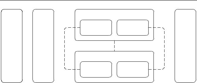
As described above, the PTSD patients in our study suffered from Panic Attacks. During and directly after a Panic Attack, there is usually a continuous worrying by the client about a new attack, which induces an acute and almost continuous form of stress. In our main studies, we attempted to mimic such stress in two ways; see also Figure 8.1.

First, in the Stress-Provoking Story (SPS) study, the participants read a stressprovoking or a positive story aloud [685]. Here, storytelling was used as the preferred method to elicit true emotions in the patient. This method allows great methodological control over the invoked emotions, in the sense that every patient reads exactly the same story. The fictive stories were constructed in such a way that they would induce certain relevant emotional associations. Thus, by reading the words and understanding the story line, negative or positive associations could be triggered. The complexity and syntactic structure of the different stories were controlled to exclude the effects of confounding factors. The negative stories were constructed to invoke anxiety, as it is experienced by patients suffering from PTSD. Anxiety is, of course, one of the primary stressful emotions. The positive stories were constructed to invoke a positive feeling of happiness.

Second, in the Re-Living (RL) study, the participants told freely about either their last panic attack or their last joyful occasion [248]. The therapists assured us that real emotions would be triggered in the reliving sessions with PTSD patients, in particular in reliving the last panic attack. As the reliving blocks were expected to have a high impact on the patient’s emotional state, a therapist was present for each patient and during all sessions. The two RL sessions were chosen to resemble two phases in therapy: the start and the end of it. Reliving a panic attack resembles the trauma in its full strength, as at the moment of intake of the patient. Telling about the last happy event a patient experienced, resembles a patient who is relaxed or (at least) in a ‘normal’ emotional condition. This should resemble the end of the therapy sessions, when the PTSD has disappeared or is diminished.

8.4 Emotion detection by means of speech signal analysis

The emotional state that people are in (during telling a story or reliving the past) can be detected by measuring various signals, as has been outlined in Chapter 2. However, more than any other signal, speech suited our purposes as:

1.Speech recordings are completely unobtrusive, see Chapter 2.

2.The communication in therapy sessions is often recorded anyway. Hence, no additional technical effort had to be made on the part of the therapists.

3.Therapy sessions are generally held under controlled conditions in a room shielded

134

8.5 The Subjective Unit of Distress (SUD)

practice baseline stress-provoking stories (SPS) study baseline

re-living (RL) study

happy

stress / anxiety

Figure 8.1: Overview of both the design of the research and the relations (dotted lines) investigated. The two studies, SPS and RL, are indicated, each consisting of a happy and a stress/anxiety-inducing session. In addition, baseline measurements were done, before and after the two studies.

from noise. Hence, the degree of speech signal distortion can be expected to be limited.

There is a vast amount of literature on the relationship between speech and emotion, as was already denoted in Chapter 2. Various speech features have been shown to be sensitive to experienced emotions; see Chapter 2 for a concise review. In this research, we extracted five characteristics of speech:

1.the power (or intensity or energy) of the speech signal; for example, see Table 2.2, Chapters 5 and 6, and [131, 469];

2.its fundamental frequency (F0) or pitch, see also Table 2.2, Chapters 5 and 6, and [131, 369, 469, 579, 696];

3.the zero-crossings rate [331, 560];

4.its raw amplitude [469, 579]; and

5.the high-frequency power [27, 131, 469, 560].

All of these characteristics have been considered as useful for the measurement of experience emotions. Moreover, we expect them to be complementary to a high extent.

8.5 The Subjective Unit of Distress (SUD)

To evaluate the quality of our speech analysis, we must compare it to an independent measure of distress. We compared the results of our speech features to those obtained from a standard questionnaire, which measured the Subjective Unit of Distress (SUD). The SUD

135

8 Two clinical case studies on bimodal health-related stress assessment

was introduced by Wolpe in 1958 and has since proven itself to be a reliable measure of a person’s emotional state. The SUD is measured by means of a Likert scale that registers the degree of distress a person experiences at a particular moment in time. In our case, we used a linear scale with a range between 0 and 10 on which the experienced degree of distress could be indicated by a dot or cross. The participants in our study were asked to fill in the SUD test once every minute; therefore, it became routine during the experimental session and has not been a stress provoking factor.

8.6 Design and procedure

In our study, 25 female Dutch PTSD patients (mean age: 36; SD: 11.32) participated of their own free will. This group of patients was chosen because we expected that their emotions could be elicited rather easy by way of the two studies, as PTSD patients are sensitive for emotion elicitation methods chosen. Hence, in contrast with traditional emotion elicitation as often conducted in research settings (cf. Chapters 3-6), true emotions were (almost) guaranteed with these studies.

All patients signed an informed consent and all were aware of the tasks included. The experiment began with a practice session, during which the participants learned to speak continuously for longer stretches of time, because during piloting it was noticed that participants had difficulty in doing this. In addition, the practice session offered them the opportunity to become more comfortable with the experimental setting. Next, the main research started, which consisted of two studies and two baseline sessions. The experiment began and ended with the establishment of the baselines, in which speech and SUD were recorded. Between the two baseline blocks, the two studies, the Stress-Provoking Stories (SPS) study and the Re-Living (RL) study, were presented. The two studies were counterbalanced across participants.

The SPS study aimed at triggering two different affective states in the patient. It involved the telling of two stories, which were meant to induce either stress or a neutral feeling. From each of the sessions, three minutes in the middle of the session were used for analysis. The order of the two story sessions was counterbalanced over participants. Both speech and SUD scores (once per minute) were collected. The RL study also involved two sessions of three minutes. In one of these, the patients were asked to re-experience their last panic attack. In the other, the patients were asked to tell about the last happy event they could recall. Again, the order of sessions was counterbalanced over participants. With both studies, problems occurred with one patient. In both cases, the data of this patient were omitted from further analysis. Hence, in both conditions, the data of 24 patients were used for further analysis.

136

8.7 Features extracted from the speech signal

Power

Amplitude

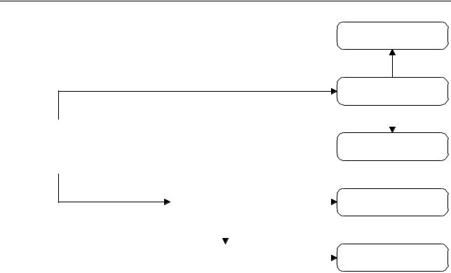
Figure 8.2: Speech signal processing scheme, as applied in this research. Abbreviations: F0: fundamental frequency, HF: high frequency.

8.7 Features extracted from the speech signal

Recording speech was done using a personal computer, a microphone preamplifier, and a microphone. The sample rate of the recordings was 44.1 kHz, mono channel, with a resolution of 16 bits. All recordings were divided into samples of approximately one minute of speech.

Five features were derived from the samples of recorded speech: raw amplitude, power, zero-crossings, high-frequency power, and fundamental frequency; see also Figure 8.2. Here, we will give a definition of these five features.

The term power is often used interchangeably with energy and intensity. In this chapter, we will follow [432] in using the term power. For a domain [0, T ], the power of the speech signal is defined:

The power of the speech signal is also described as the Sound Pressure Level (SPL),

137

8 Two clinical case studies on bimodal health-related stress assessment

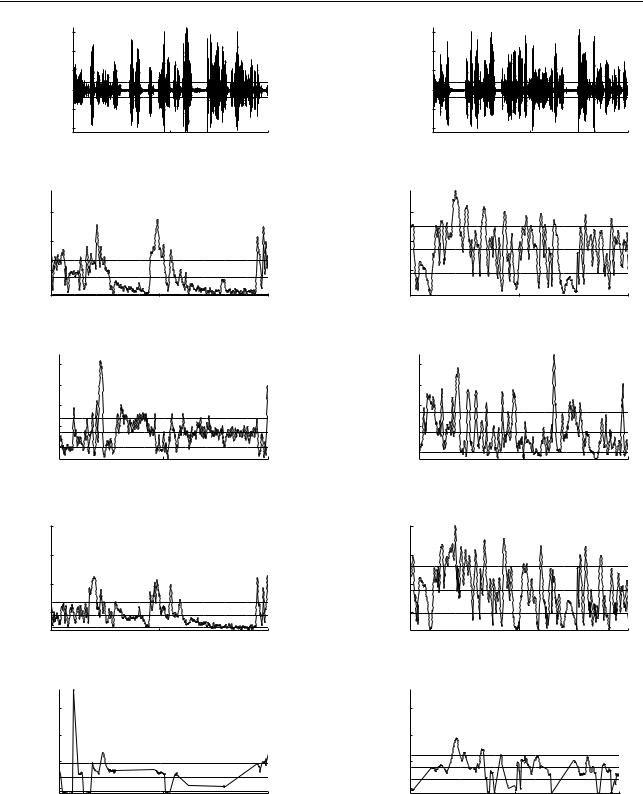
Figure 8.3: A sample of the speech signal features of a PTSD patient from the re-living (RL) study. The dotted lines denote the mean and +/- 1 standard deviation. The patient’s SUD scores for this sample were: 9 (left) and 5 (right). Power (dB) (top) denotes the power and the High Frequency (HF) power (dB) (bottom).

138

8.7 Features extracted from the speech signal

calculated by the root mean square of the sound pressure, relative to the auditory threshold P0 (i.e., in deciBel (dB) (SPL)). Its discrete equivalent is defined as [554]:

The third feature that was computed was the zero-crossings rate of the speech signal. We refrain from defining the continuous model of the zero-crossings rate, since it would require a lengthy introduction and definition (cf. [552]). This falls outside the scope of this chapter.

Zero crossings can be conveniently defined in a discrete manner, through:

where N is the number of samples of the signal amplitude x. The I {α} serves as a logical function [331]. An example of this feature is shown in Figure 8.3c. Note that both power and zero-crossings are defined through the signal’s amplitude x; see also Figure 8.2, which depicts this relation

The fourth feature that was extracted is the high-frequency power [27]: the power for the domain [1000, ∞], denoted in Hz. In practice, ∞ takes the value 16, 000. To enable this, the signal was first transformed to the frequency domain; see also Figure 8.3d. This is done through a Fourier transform X(f ) (see also Figure 8.2), defined as [432]:

with j representing the √−1 operator. Subsequently, the power for the domain [F1, F2] is defined as:

For the implementation of the high-frequency power extraction, the discrete Fourier transform [432] was used:

N −1

X(m) = N1 X x(n)e−j2πnm/N , (8.6)

n=0

139

8 Two clinical case studies on bimodal health-related stress assessment

with j representing the √−1 operator and where m relates to frequency by f (m) = mfs/N . Here, fs is the sample frequency and N is the number of bins. N typically takes the value of the next power of 2 for the number of samples being analyzed; for example, 640 for a window of 40 msec. sampled at 16, 000 Hz. The power for the domain [M1, M2], where f (M1) = 1000 Hz and f (M2) = fs/2 (i.e., the Nyquist frequency), is defined by:

The fundamental frequency (F0) (or perceived pitch, see Table 2.2) was extracted using an autocorrelation function. The autocorrelation of a signal is the cross-correlation of the signal with itself. The cross-correlation denotes the similarity between two signals, as a function of a time-lag between them. In its continuous form, the autocorrelation r of signal x at time lag τ can be defined as [53]:

In the discrete representation of Eq. 8.8, the autocorrelation R of signal x at time lag m is defined as [607]:

n=0

where N is the length of the signal. The autocorrelation is then computed for each time lag m over the domain M1 = 0 and M2 = N − 1. The global maximum of this method is at lag 0. The local maximum beyond 0, lag mmax, represents the F0, if its normalized local maximum Rx(mmax)/Rx(0) (its harmonic strength) is large enough (e.g., > .45). The F0 is derived by 1/mmax. See Figure 8.3e for an illustrative output of this method.

Throughout the years, various implementations have been proposed for F0 extraction; for example, [53, 607]. See Table 2.2 for a discussion on speech signal processing and on F0 extraction in particular. In this research, we have adopted the implementation as described in [53]. This implementation applies a fast Fourier transform (see also Eq. 8.4 and Eq. 8.6) to calculate the autocorrelation, as is often done; see [53, 607] and Table2.2. For a more detailed description of this implementation, we refer to [53].

Of all five speech signal features, 13 statistical parameters were derived: mean, median, standard deviation (std), variance (var), minimum value (min), maximum value (max), range (max − min), the quantiles at 10%(q10), 90%(q90), 25%(q25), and 75%(q75), the inter-quantile-range 10% − 90% (iqr10, q90 − q10), and the inter-quantile-range 25% − 75%

140