Jessica Gurevitch, Samuel M. Scheiner, and Gordon A. Fox - The Ecology of Plants - 2002 / The Ecology of Plants Jessica Gurevitch, Samuel M. Scheiner, and Gordon A. Fox; 2002 / Ch 07

118 Chapter 7

population growth model tailored for plant populations was published in 1974 by Harper’s student Jose Sarukhán, working with Madhav Gadgil (Sarukhán and Gadgil 1974). In the decades since this early work, there has been an explosion of work in plant population ecology; hundreds of papers are now published annually. Harper’s students have in turn trained many plant ecologists

all over the world. Sarukhán, for example, returned to Mexico and helped develop the Universidad Nacional Autónoma de México into an important center for ecological research, especially on plants.

Ecologists often distinguish between densitydependent and density-independent population growth. Some factors affecting population growth depend on the density of a population. For example, competition might be important in a crowded stand of plants, but much less important when there are greater distances between individuals. Thus, competition is usually thought of as a den- sity-dependent factor. By contrast, if 10% of all juveniles were killed by a severe storm, regardless of population density, ecologists would say that the weather is acting as a density-independent factor.

Although this distinction between density dependence and density independence seems simple enough, nature is often more complicated. If a severe storm kills 10% of all the individuals not growing in sites protected from high winds, and protected sites are in limited supply, is the mortality density-dependent or densityindependent? Clearly, the distinction between the two types of mortality is not very meaningful in such cases. Nevertheless, this distinction is often quite useful,* and in any case density independence is a good starting point for thinking about population growth.

This distinction must be applied cautiously to plants. In discussing the assessment of competition, Harper (1977) pointed out that the average density over a whole plant population is not the important quantity to measure. Because plants are sessile, they usually compete only with their neighbors, not with more distant plants in the same population (see Chapter 10). Thus, when assessing competition, one needs to think of density dependence on a very localized scale. Other spatial scales may be important for other phenomena—for example, many pathogens can disperse over considerable distances, so average density over a larger area may be a useful quantity to measure to understand the progress of disease in a population. A more general way to categorize these dif-

* Many important scientific ideas are like this: valuable in one context but not in another. That is because such ideas are simplified descriptions of nature— useful but limited models of patterns or processes (see Chapter 1).

ferent kinds of phenomena would be to distinguish between changes in the population that depend on interactions among individuals (such as competition) and changes that do not require such interactions. Because ecologists use the terminology of density to describe population change, we will use it here as well.

This chapter concerns density-independent changes in population size. We discuss density-dependent changes in populations in Chapters 10 and 11.

Some Issues in the Study of Plant

Population Growth

What controls the growth and decline of plant populations? Change in population size is determined by the numbers of births and deaths, plus the number of individuals immigrating into the population, minus the number emigrating from the population. Ecologists usually get data on changes in population size by conducting regular censuses—say, by counting individuals every year or every week. If we think of the first census as occurring at time t, and the next census as occurring at time t + 1, then we can describe the change in population size as

Here the n’s are the population sizes at sequential censuses. For example, if we were tracking a population of Pinus ponderosa (Ponderosa pine, Pinaceae), nt would be the number of individual trees in the first year of our census, and nt+1 would be the number of trees in the following year. Bt is the number of births between the two censuses, Dt the number of deaths, It the number of individuals arriving (immigrating) from other populations, and Et the number dispersing away (emigrating) from the population.

The relationship in Equation 7.1 may seem to be a truism. Though simple, it is a useful starting point because it helps us to focus on some major factors affecting plant population growth. It also points to some major differences between plant and animal populations and to some major conceptual problems in plant ecology.

Equation 7.1 implies several equivalent ways in which plant population size can be affected. It implies, for example, that the same population growth can be assured by increasing the number of births or by decreasing the number of deaths. As we will see in much of the rest of this chapter, life is not generally so simple unless all of the individuals in a population are demographically equivalent, and that is rarely the case. Large plants usually have different effects on the population than small ones, and old plants usually have different effects than young ones. Therefore, adding x births is not usually equivalent to reducing the number of deaths by x.

But Equation 7.1 raises still more issues. What exactly do we mean by “birth” and “death” in plant populations? That depends on whether we mean births and deaths of genetically distinct individuals (genets) or of individuals that may be physiologically independent but are not necessarily genetically distinct (ramets; see Figure 5.8). One useful way to keep this distinction straight is to remember that every new genet is also a new ramet, but the reverse is not necessarily true: a new (potentially) physically independent individual is not necessarily a new genetic individual.

New genets are formed by the fertilization of an ovule and the maturation of the resulting seed (see Chapter 8). In plant species that never spread clonally (such as most annual herbs), each genet is a single ramet. Plant ecologists usually think of birth as occurring either when the seed is mature (i.e., the embryo is fully formed) or when the maternal plant sheds the seed. Seed germination is not considered birth because seeds are already new individuals—physiologically independent and (usually) genetically distinct from their parents long before they germinate. Moreover, they often spend a substantial amount of time, sometimes years, living in the soil before germination. Plant populations whose seeds have such a dormant phase are said to have a seed bank.

Many plants can spread clonally (also called vegetatively) by producing structures that contain tissues capable of producing an entire new plant, which is genetically identical to the parent. In these species, each genet is usually made up of multiple ramets, some of which may be physiologically independent from one another. Thus, discussing births and deaths in populations of these species means that first we must decide whether we are studying change in the number of genets or in the number of ramets. Studies of genet number would use a definition like the one above: newborns would consist only of new seeds. Studies of ramet number would count all new individuals, including both new seeds and new shoots, because all of them are new ramets. Which definition is best? That depends on the questions one asks.

This distinction between ramets and genets affects the way we think about dispersal between populations (the It and Et terms) as well. Most mature plants are ses- sile—rooted in place—but (by the above definition) seeds are certainly plants, and they are usually mobile. Similarly, pollen grains are plants that are usually mobile (a pollen grain is the male gametophyte of gymnosperms and angiosperms, and is multicellular and genetically different from the sporophyte plant that produced it; see Chapter 8). It should not be surprising, therefore, that seeds and pollen, and their dispersal, have been and continue to be the subject of much ecological research. But some plants can disperse by clonal fragmentation as well. Many cholla cacti (Opuntia spp., Cac-

Population Structure, Growth, and Decline 119

taceae Figure 7.1), for example, lose joints that are then moved by animals or runoff from storms; these may take root and grow into mature plants. At the other end of the moisture availability gradient, while dispersal of clonal fragments is rare in marine angiosperms such as Zostera spp. (eelgrasses, Zosteraceae; Barrett et al. 1993), it may be quite important in the establishment of new populations. Since most living plant tissues can, at least potentially, generate entirely functional new plants, dispersal by clonal fragmentation may be widespread.

Dispersal by clonal fragmentation has another implication. Seed dispersal means that an individual immigrating to one population must be emigrating from another. Clearly this is not so with dispersal by fragmentation: while the fragment itself may leave one population and move to another, the rest of the genet from which it was derived may stay put.

This does not mean that dispersal by fragmentation is a “free lunch.” Indeed, it has an obvious consequence:

Figure 7.1

Many Opuntia cacti—especially the chollas, which have cylindrical joints—disperse partly by clonal fragmentation; some of the fragments root and establish new ramets. Opuntia fulgida, shown here, is known as “jumping cholla” because its joints very readily detach from the parent plant; unwary people walking by (including the authors) have been unpleasantly surprised by this plant! (Photograph by S. Scheiner.)

120 Chapter 7

the fragmenting genet is packaged into smaller ramets. Since the survival and fecundity of ramets usually depend at least in part on their size, it is possible that clonal fragmentation might eventually affect the survival of the genet as a whole. It is an open question how the population dynamics of ramets and of genets affect one another.

Population Structure

The preceding discussion points to an important conclusion: When we study plant populations, we usually need to pay attention not only to the total number of individuals in a population, but to the classes of individuals and the relative frequencies of each class in the population as well. These classes are usually defined by age, life history stage (e.g., seed, seedling, sapling, canopy tree), size (e.g., 0–2 cm, 2–4 cm, >4 cm tall), or some combination of these categories. The population structure is a description of the relative frequency of each class (Figure 7.2).

Information about population structure is important for two reasons. First, different kinds of individuals have different effects on population growth. Adding 100 seeds to a population of the giant Sequoia sempervirens (California redwood, Taxodiaceae), for example, would obviously have a very different effect on the growth of the population than adding 100 mature redwood trees. If you were asked to census a tree population, you would almost certainly count seeds, seedlings, saplings, and mature trees as different classes, and you might make even finer distinctions. Ecologists need to know what kinds of individuals are in a population as well as their numbers. This is generally true for both animal and plant populations.

The second reason we need to know about population structure is particular to plants. Because of their extreme phenotypic plasticity, individual plants can vary over orders of magnitude in size, shape, physiological status, and consequently, in their importance for population growth (see Chapter 5). Animals certainly vary in their size and contribution to population growth as well. But we can often predict the vital rates of an animal—its reproductive rate and its chance of surviving—if we know only its age. Many animal populations (especially mammals and birds) can thus be thought of as age-structured. To describe such populations, we need to know how many individuals are in each age group. The methods used for the study of these populations are age-based, requiring only information on the population’s age structure. Age-structured populations have another convenient property: they progress in only one direction. A bear that is x years old now will either be dead or age x + 1 next year.

In most plant populations, stage—a category based on size, physiology, or developmental status, such as

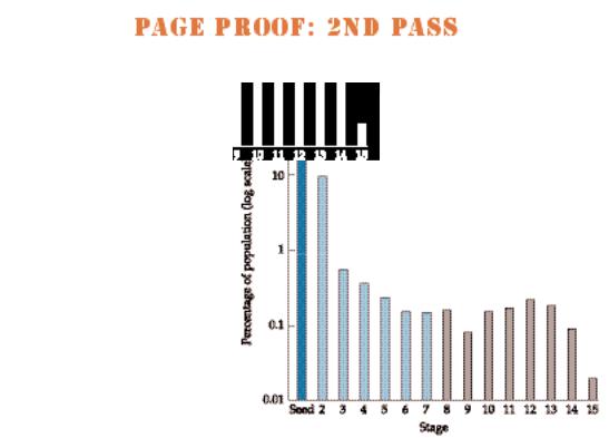
Figure 7.2

Stage structure of a population of Pentachlethra macroloba (Fabaceae), a tropical tree species, at Barro Colorado Island, Panama. Here, the stage classes above seed are based on size. Classes 2–7 (seedlings; light green) are in increments of 50 cm in height. Subsequent classes are based on diameter at breast height (DBH): class 8 = 2–5 cm, class 9 = 5–10 cm, class 10 = 10–20 cm, classes 11–14 are in 20 cm increments, and class 15 > 100 cm. Thus 88% of the population consists of seeds and 9% of seedlings 0–50 cm in height. The remaining stages (gray bars) comprise only 3% of the population. (After Hartshorn 1975.)

seed, seedling, juvenile, small individual, large individ- ual—plays a stronger role in determining demographic performance than age; therefore, plant populations are generally thought of as stage-structured (see Figure 7.2). This should be obvious in the case of reproductive output because the number of flowers and fruits usually depends on plant size. Survival and subsequent growth usually also depend on plant size more than on age. Older plants are usually larger, but in most plants there is so much variation in the sizes of individuals of a given age (Figure 7.3) that it is often more useful to use stage-based methods than age-based methods to study plant demography.

That said, we hasten to add that chronological age can be important to know in plants for several reasons. Age is quite important in an evolutionary context; for example, if we want to understand how the genetic composition of a population changes over time, we need information about the ages of individuals. Similarly, if we want to study the evolution of life history traits (see Chapter 9), we often need information about the ages of individuals. As we will see in several examples in this chapter, age is sometimes an important determinant of

Figure 7.3

The average relationship between age and size in Pinus palustris (longleaf pine, Pinaceae) in the southeastern United States. The data show the average number of plants per acre of a particular size, given the age of the stand. Longleaf pine frequently grows in such even-aged stands. (After Forbes 1930.)

survivorship (the chance of surviving) and fecundity (the number of offspring contributed to the next generation). But age alone is not a very good predictor of these vital rates in plants; stage information is usually needed as well.

old seeds have a different chance of germinating than two-year-old seeds, and a different chance of surviving as viable seeds in the seed bank. Similarly, in Cypripedium acaule (pink ladyslipper orchid, Orchidaceae; Figure 7.5), the survival of corms from year to year depends on their age, and the survival of dormant plants from year to year depends on the number of years they have been dormant.

While age can be important, it is frequently impossible to determine a plant’s age. Although many temper- ate-zone trees do produce reliable annual growth rings, most other plants—both herbs and woody plants—do not. Unless we are working with marked individuals of known age, then, we usually do not know the ages of plants (but see the discussion of long-lived plants on page 133).

Some population structure issues special to plants

Why are plants so much more variable in their population structure than animals? A major reason is their modular growth form: an individual plant is a system of repeated units (nodes, lateral organs, and internodes: see Chapters 5 and 8). This modularity means that plants have very flexible growth patterns. It also means that they can lose large areas of their bodies and still survive. In other words, plants can actually shrink from year to year. In the ladyslipper orchid, for example, adults may not appear aboveground in some years (see Figure 7.5).

Stage structuring makes life complicated for plant ecologists. As mentioned above, when dealing with animals, one can be certain that in a year, all individuals now

Cypripedium acaule

Figure 7.5

Life cycle graph of Cypripedium acaule (pink ladyslipper, Orchidaceae), a terrestrial orchid from eastern North America. After germination, a corm develops underground for at least two years; subsequently, each plant produces zero, one, or two leaves every year. Mature C. acaule can produce additional ramets, treated in this study as new individuals; this vegetative reproduction is not shown here. (Photograph by S. Scheiner.)

x years old will be either dead or a year older. Even in many stage-structured animal populations, individuals can never move to an earlier stage—frogs do not become tadpoles. There are few such prohibitions in plants. Once germinated, a plant can never become a seed, but in most plant species established plants can grow, stay the same size, or shrink (Figure 7.6). Even trees, which we often think of as always growing larger, lose branches and sections of their trunks. Consequently, plant ecologists need

to keep track of many stages and possible transitions between them.

Sources of Population Structure

Individuals within plant populations vary in many characteristics, including size, morphology or developmental status, genotype, and physiological status. Size is the most commonly studied factor structuring plant populations. Size can be measured in several ways: as a quan-

tity such as weight or height or as the number of modules (e.g., branches, tillers in a grass, or leaves) a plant has. Tree size is often measured as diameter at breast height (DBH); curiously, “breast height” is defined as 1.3 meters in some countries and 1.4 in others. Morphological or developmental status is usually important in structuring populations: how many individuals are seeds, how many seedlings have become established, how many plants have become reproductively active? Genetic variation is often important in structuring populations, and physiological status is probably often important as well.

This list of categories may seem a bit overwhelming, but categories such as size, morphology, age, genotype, and physiological status are important for population studies only if there are demographic differences among the classes. For example, it might be easy to measure the difference in size between 30-, 60-, and 90-cm DBH trees of the same species, but it may not be useful to use these size differences as size classes if the trees of each size did not differ from the other sizes in their chances of survival, growth, or reproductive output.

Currently, there are real limits to our abilities to measure this variation, to tell how important it is in structuring a particular population, and to perform appropriate computations. Consequently, most ecological studies today concentrate on only one or a few of these categories of variation. Put differently, we know that reality is much more complex than our demographic analyses.

Studying Population Growth and Decline

Is a population growing or declining, and at what rate? This might seem like a simple question to answer: compare the number of plants last year (call it nt) with the number this year (call it nt+1). The rate of change in population size is then n t+1/nt. If the population is growing, this ratio is greater than 1; if the population is declining, the ratio is less than 1.

Unfortunately, life is this simple only when there is no population structure. Certainly it is true that if nt+1 > nt, there are more plants now than there were last year. But in a structured population—that is, in most plant populations—individuals of different classes make different contributions to future population growth. This means that their short-term effects can differ from their long-term effects on the population, and we need to be able to ask about both kinds of effects.

Consider a population of a long-lived tree species. The oldest trees have a period of senescence that lasts up to several decades, during which they do not flower but slowly lose limbs and experience heartwood rot. Young trees cannot flower until they are several decades

Population Structure, Growth, and Decline 123

old. Thus neither very old nor very young trees are reproducing, so a population of 100 very old or very young trees will simply decline in number as some die and none reproduce.

Now imagine that year-to-year survival rates are the same among young and old trees, and compare a population composed entirely of old trees with one composed entirely of young trees. In the short run, both populations will decline at the same rate. But over time, this will not be true, because the surviving trees in the young population will eventually reach maturity and begin reproducing, so the population will grow. By contrast, the old population will disappear. Therefore, studies of population growth and decline in plants must take into account the structure of the population and look at both long-term and short-term growth.

Life Cycle Graphs

To learn how population structure affects population growth, we need a picture of how individual plants can shift from stage to stage between censuses. Life cycle graphs such as those in Figures 7.4 through 7.7 provide useful summaries of information about transitions between stages. Each node in a life cycle graph represents a stage. Note that some stages are defined by developmental status (e.g., seeds and dormant individuals), while others are defined by their size or age within a developmental stage. Arrows between stages describe “transitions” between those stages—survival and reproduction—during the interval between censuses.

Let’s look at the life cycle graph for Coryphantha robbinsorum (pincushion cactus, Cactaceae) (Figure 7.7). (This endangered cactus species will be used as an example throughout the next few sections of the chapter.) The arrow from large juveniles to adults represents the probability (P) of a large juvenile at one census becoming an adult by the next census. The self-loops—arrows from a node to itself—represent the probability of remaining in the same stage. Thus, the arrow from small juveniles to small juveniles in Figure 7.7 represents the probability that a small juvenile at one census will still be a small juvenile at the next census.

The arrow from adults to small juveniles in Figure 7.7 needs a more careful interpretation, which points to an important lesson about life cycle graphs and the matrix models that can be derived from them. This arrow refers to the number of small juveniles produced by the adults. Biologically, we know that every individual starts as a seed, and that there is generally some time between seed maturation and germination (there are a few viviparous plant species that germinate right on the maternal plant, but Coryphantha is not one of them). A complete biological diagram of the life cycle would include these steps. But we are trying to describe

the demography of the life cycle as examined in a real field study. Since this species has no seed bank and the censuses are annual, no individuals in the seed class could have been counted unless the census were timed to include them. To represent Coryphantha demography as measured, then, we need to estimate fecundity:

F = (rate of seed production) × (chance of seed survival) × (chance of germination) × (chance of seedling surviving to the first census) =

(the rate at which adults one year produce small juveniles the next)

If we wanted to study the seed stage per se, we would need censuses that were timed differently, and possibly more frequent censuses. This may seem like a quibble, but it turns out that the number of classes we include

Coryphantha robbinsorum

Figure 7.7

Life cycle graph of Coryphantha robbinsorum (pincushion cactus, Cactaceae), an endangered cactus from Arizona and Sonora, Mexico. As this species has no seed bank and plants were censused annually, the graph does not include a seed stage. The transition between adults and small juveniles is thus the product of (rate of seed production) times (chance of a seed surviving) times (chance of germination) times (chance of a seedling surviving to the first census). (Data from Schmalzel et al. 1995; photograph courtesy of U.S. Geological Survey, Phoenix, AZ.)

in a life cycle graph or matrix model can greatly affect most calculations for which the graph or matrix model is subsequently used.

Once we have a life cycle graph, we can then use field data to estimate values for the various transitions (Figures 7.4–7.7; Box 7A). Often it is impossible to observe all of the transitions directly using the same indi-

Coryphantha robbinsorum is a small, cluster-forming cactus found on limestone outcroppings in southern Arizona and adjacent Sonora, Mexico. Schmalzel et al. (1995) marked plants at three sites on a hill and followed their growth, reproduction, and survival for a five-year period.

Because adults (plants that had flowered at least once), small juveniles (plants smaller than 11 mm in diameter), and large juveniles had significantly different chances of survival and reproduction, the authors used these and seeds as their stage classes. Since C. robbinsorum has no seed bank (see Figure 7.7) and the censuses were annual, we re-analyzed the authors’ data with

a model that does not include a seed stage. The data can be used to create matrix models for each of the three sites:

Analysis of these matrices reveals that the population at site C is growing, because λ1 = 1.12. At the other two sites, the population is stable or declining slowly: λ1 = 0.998 at site A and λ1 = 0.997 at site B. The stable stage distributions differ among these plots, as Figure 7.9 shows. Most notable is the predicted scarcity of large juveniles at sites A and B. The plots also differ in the rates at which they approach the stable distribution. Sensitivities are shown in Table 7.2, elasticities in Figure 7.10, and reproductive values in Table 7.1.

viduals. For example, it is difficult to use the same individuals to estimate the survival and germination rates of seeds as well as subsequent transitions, because seeds usually cannot be marked, and even when they can be, accurate censusing usually requires digging them up— which can certainly bias their future chances of surviving or germinating!

In a large study of Collinsia verna, Susan Kalisz and Mark McPeek (1992) addressed this problem by estimating seed survival rates destructively but independently from their estimates of the vital rates of aboveground plants (see Figure 7.4). They were able to do so because C. verna grows in very large populations, making it possible to randomly select separate areas for studying aboveground and belowground demography.

On the other hand, in the ladyslipper orchid study (see Figure 7.5), Margaret Cochran and Stephen Ellner (1992) were forced to make several assumptions about mortality rates in dormant plants and seeds. It would have been more satisfactory to observe the belowground events directly, but this would have destroyed study areas, and might have added to the effects of poaching on these orchids. There are no simple or general solutions to this problem.

Matrix Models

How do the rates of survivorship and fecundity affect the growth of a population as a whole? Which stages have the strongest effects on population growth? Questions like these are important in many contexts, including conservation biology (on which stages should we concentrate protection efforts?), population ecology (which stage is most likely to limit population growth?), and evolution (on which stage can natural selection have the greatest effect?).

One approach to answering such questions is to use estimated survivorship and fecundity rates to model the population’s growth rate, using matrix demographic methods developed over the past two decades. These models can be used to ask how the population growth rate changes as the specific survivorship and fecundity rates in each class change. All of the information needed for this method is contained in the life cycle graph.

To see this, consider the Coryphantha example (see Figure 7.7). The life cycle graph tells us that small juveniles are produced by adults at a rate F (as noted above, F is a composite of several factors). For convenience, we number the stages from 1 to 3, so that every symbol we use can be interpreted. Thus n1 means the number of small juveniles, n2 the number of large juveniles, and n3 the number of adults. Each transition has two sub- scripts—the first refers to the stage this year, and the second to the stage last year. Thus P11 is the probability of remaining a small juvenile, P32 is the probability of a

Population Structure, Growth, and Decline 125

large juvenile becoming an adult, and so on. Using these symbols, we can write an equation for the number of small juveniles in year t + 1:

In other words, the number of small juveniles this year is the sum of the individuals that remain small juveniles plus new juveniles; that is, the number of small juveniles last year times the chance that they survived as small juveniles, plus the number of adults last year times their rate of production of small juveniles.

Similarly, the number of large juveniles is given by

That is, the number of large juveniles this year is the number of small juveniles last year times the chance that they became large juveniles, plus the number of large juveniles last year times the chance that they remained large juveniles.

Finally, the number of adults is

The number of adults this year is the number of large juveniles last year times the chance that they became adults, plus the number of adults last year times the chance that they survived as adults.

A transition matrix model is a compact way of writing the same thing. The matrix arranges the coefficients from the life cycle graph (the F’s and P’s, shown as a matrix in the middle of Equation 7.5). This matrix thus represents the survivorship and fecundity rates. Next a vector is assembled consisting of the number of individuals of each stage; in Equation 7.5, this is the column on the right-hand side. To obtain a vector of the number of individuals in each stage next year—the column on the left-hand side of Equation 7.5—we multiply the vector by the matrix. In Box 7B, we explain the rules for multiplying the vector by the matrix. A matrix model of the life cycle graph in Figure 7.7 can thus be written as

More general rules for manipulating matrices are given in Caswell (2001).

The principal reason for using matrices is that there are standard rules for manipulating them, and these rules make it much easier to draw some important ecological conclusions about the population. If we assume (for the moment) that the birth and survival probabilities (the coefficients) stay constant (so that each year we multiply the population vector by the same matrix), we can find

To find the second element in next year’s vector (the number of large juveniles), repeat this process, but multiply each of the elements of this year’s vector by the coefficients in the second row of the matrix.

Another useful way of thinking of the matrix is that it describes the transitions in “from-to” form. The matrix element in the ith row and jth column always refers to the transition from the jth stage to the ith stage—from the “column-number” stage to the “rownumber” stage.

•The shortand long-term population growth rates

•The population structure at any time in the future

•The reproductive value of each age or stage class. Roughly speaking, the reproductive value of an individual in class x is its expected contribution to future population growth. In other words, reproductive value is a way of evaluating the relative demographic importance of the different classes

•The sensitivity and elasticity of population growth to changes in the specific probabilities of survival and reproduction. Sensitivity tells us how absolute changes (e.g., how adding 0.01 to a survivorship coefficient) in the survival and fecundity of each class would affect population growth rates; elasticity tells us how proportional changes (e.g., how increasing a survival coefficient by 1%) would change the population growth rate.

•The relationship between the ages of individuals and their stages

Matrix models and the estimates of growth rates, reproductive value, sensitivity and elasticity that they provide are important tools in evolutionary ecology, conservation biology, and applied ecology.

Analyzing Matrix Models

How do we get all of this information from matrix models? In this section we introduce some major ideas used in analyzing these models. The basic method used to analyze matrices depends on an important observation: if we repeatedly multiply the population vector—the vector of the number of individuals of each stage—by the transition matrix, after a while the population vec-

tor attains a stable structure or stable stage distribution, at which point the proportion of individuals in each class stays constant each generation, although the population keeps growing. This observation implies that, at least once the population has reached its stable structure, we can multiply the population vector by a single number (a scalar) rather than by the entire matrix and get the same result as if we were multiplying by the matrix.

How do we find this number? Mathematically, we are looking for a number, which can be denoted by λ (the Greek letter lambda), based on the equation A x = λ x, where A is the transition matrix and x is a vector. (In this chapter we will use standard mathematical notation: capitalized boldfaced symbols, such as A, are matrices, and lowercase boldfaced italic symbols, such as x, are vectors.) It is always possible to find such numbers (the values for λ) for transition matrices; this is almost always done numerically on a computer. Numbers that can play this role are called eigenvalues or characteristic values. Every such number λ has a corresponding population vector x, called an eigenvector or characteristic vector. For a population with N stages, the transition matrix has N rows and columns. There are also N eigenvalues. Each eigenvalue has a corresponding eigenvector. In most cases, all of the eigenvalues are distinct, although under some circumstances there are pairs of duplicated eigenvalues.

The number λ tells us some important things about a population. If λ > 1, the population is growing, while if λ < 1, it is declining in number. The population remains at a constant size only in the special case that λ = 1. But what are these eigenvalues and eigenvectors? The eigenvalues are components of the population’s