Jessica Gurevitch, Samuel M. Scheiner, and Gordon A. Fox - The Ecology of Plants - 2002 / The Ecology of Plants Jessica Gurevitch, Samuel M. Scheiner, and Gordon A. Fox; 2002 / Ch 12

234 Chapter 12

PAGE PROOF: 2ND PASS

A very confusing array of terms has developed to describe communities. Sometimes the same term is used in different ways by different ecologists, while in other cases different terms are given to the same concept. Here we describe a recently proposed scheme to define these terms.

This scheme defines groups of species based on three criteria: geography, phylogeny, and resource use, as shown in the accompanying figure. Geography in this scheme defines communities, sets of organisms living in the same place at the same time. Phylogeny is the pattern of relationships among species (or higher taxa) based on evolutionary ancestry. Phylogeny defines taxa, sets of organisms that share a common ancestor. Resource use defines guilds, sets of organisms that use biotic or abiotic resources in a similar way. The term “guild” is taken from animal ecology, but has been used by plant ecologists as well.

Plant ecologists often use the term functional group to describe a concept related to the guild. Functional groups can be defined in a variety of ways, depending on the application, but these definitions are all based on a set of traits that identify functionally similar species. The traits used to identify functional groups can be chosen informally or based on formal mathematical algorithms. Ecologists have used the concept of functional groups in a variety of contexts, including studies of the relationship between productivity and diversity (see Chapter 14) and attempts to reduce the number of types of plants that must be taken into account in global climate modeling. Extensive recent reviews of the concept of plant functional groups and ecological applications of this concept are provided by Lavorel and Cramer (1999) and Woodward and Cramer (1996).

Intersections of the sets described by the terms above define more narrow distinctions. The intersection of geography and phylogeny defines assemblages, groups of related organisms liv-

PAGE PROOF: 2ND PASS

fication schemes (see Table 16.3). An association was defined as a particular community type, found in many places and with a certain physiognomy and species composition; modern usage is not much different (e.g., Table 16.3 refers to the juniper-sage woodland association). The term formation was originally used to denote a regional climax community; modern usage is generally more specific, referring to a physiognomic subtype.

In practice, the boundaries of plant communities are usually defined operationally, based on changes in the abundance of the dominant, or most common, species. Sampling is then confined within those boundaries. A stand is a local area, treated as a unit for the purpose of describing vegetation. Typically, a number of stands are used to sample the presence and abundances of species as well as associated environmental variables. Based on data from a number of stands, the community can be characterized.

Only in special cases (e.g., islands, ponds, forest preserves surrounded by suburban development, vacant lots) are community boundaries defined easily. Even then, the movement of organisms and the transport of matter by wind and water make their boundaries fuzzy. Ecologists, therefore, are often of two minds when dealing with communities. On the one hand, we recognize that their boundaries are fuzzy; on the other hand, we often need to define discrete entities for convenience of analysis. Typically, plant ecologists define a community based on the relative uniformity of the vegetation and use their knowledge of species biology to decide when they are moving from one community to another.

Ecologists based in different countries, educated in different historical traditions, tend to view communities in somewhat different ways. In particular, ecologists in continental Europe were historically influenced by the floristic-sociological approach, most extensively developed by Josias Braun-Blanquet (see Chapter 16). This approach emphasizes the discreteness of communities. In contrast, most ecologists in English-speaking countries have been more strongly influenced by the history described in the following paragraphs; as a result, they tend to think of communities as blending continuously into one another. These distinct ways of thinking are becoming less prominent as a result of increased travel and communication among ecologists worldwide.

The History of a Controversy

Within plant ecology, there has been, and still is, a range of views on the nature of communities. The extremes are sometimes labeled the Gleasonian and Clementsian views, named after Henry A. Gleason and Frederic Clements, their first major proponents in the Englishspeaking world. These two extreme viewpoints differ in the importance they ascribe to biotic versus abiotic factors and predictable versus random processes in shaping community structure. Today, most ecologists hold

Community Properties 235

a middle ground between these viewpoints, and to a large extent have moved beyond both of them.

The Clementsian view was the majority view among English-speaking plant ecologists during the first half of the twentieth century. Clements saw plant communities as highly organized entities made up of mutually interdependent species. In his view (Clements 1916), communities are superorganisms—the analogue of individual organisms—that are born, develop, grow, and eventually die. Succession, in this

view, is analogous to the process of development and growth; its trajectory and end point are highly predictable (Clements 1937). Two of the hallmarks of the superorganism concept were the presence of very tight linkages among species within communities and cooperation among the species in a community for the benefit of the function of the entire community.

Even at the height of Clements’s influence, many ecologists held more

moderate views. This version of Clementsian ecology asserted only that species interactions such as competition, mutualism, and predation are important in determining community structure. Clements himself acknowledged the effects of abiotic factors such as site history and soils in determining community composition. He focused on the idealized nature of communities, and saw them as spatially distinct, with one superorganism complex giving way to another with a very different collection of species. His major focus was on the nature and development of the community as a superorganism, however, rather than on the boundaries between communities. Some ecologists of the day accepted a more moderate version of this view, which admits that communities are not entirely discrete, but still divides them into nonarbitrary groups with recognizable boundaries.

In striking contrast to Clements, Gleason believed that communities are the result of interactions between individual species and the environment (biotic and abiotic factors) in combination with chance historical events. Each species has its own environmental tolerances and thus responds in its own way to environmental conditions (Gleason 1917, 1926). The implication of this belief was that along an environmental gra-

dient, different species would have their boundaries at different places. Not only were communities not tightly linked superorganisms, but defining the collection of species living together in a particular place as a community was an arbitrary human construct.

236 Chapter 12

PAGE PROOF: 2ND PASS

According to the Gleasonian view, within the range of environmental conditions a species can tolerate, chance events determine whether a species is actually found in a given location. At the local scale, chance dictates whether a seed happens to get to a particular spot. On larger scales, the chance events of history play a strong role. For example, species in the family Cactaceae (the cacti) are found in the desert communities of the Americas because the family originated in this region, while deserts elsewhere have no cacti (except where they have been recently introduced by humans). Furthermore, the mix of species changes from place to place as one moves across the landscape. The Gleasonian viewpoint posits gradual changes in community composition as opposed to abrupt boundaries between communities unless there are abrupt and large environmental boundaries. A more moderate viewpoint was that some identifiable community types exist, but that these tend to blend into other community types.

Clementsian ecologists were not receptive to Gleason’s ideas. While Gleason’s work was well known, it failed to influence many plant ecologists until after Clements’s death in 1945. Why Clements’s views held sway for so long is not fully understood. Clements was said to have an extremely strong personality that could dominate scientific meetings. Given the very small number of plant ecologists active during the first half of the twentieth century, perhaps this alone was sufficient. Gleason, finding little interest in his ideas, abandoned his work in plant ecology by 1930 and spent the rest of his career as a taxonomist.

Not until the 1950s did the separate but almost simultaneous work of John T. Curtis and Robert H. Whittaker convince many ecologists that Gleason’s views were largely correct. Curtis and his students mapped the vegetation of Wisconsin and looked at how species’ optima and ranges were distributed along environmental gradients (Curtis 1959). The Clementsian theory predicts that species optima and ranges should show distinct groupings, whereas the Gleasonian theory predicts independence of optima and ranges. The researchers found just such independence; each species had a different set of environmental tolerances (Figure

12.1). A key innovation that contributed to this study was the development of ordination, a set of techniques for describing patterns in complex vegetation; we discuss ordination in detail in Chapter 16.

Whittaker (1956) also demonstrated that Gleason was right about the nature of boundaries between communities. One of the most striking patterns one encounters going up an elevational gradient is the dra-

Environmental gradient

Figure 12.1

Change in the importance of various tree species along a moisture gradient in Wisconsin. Importance was measured as the sum of the relative cover, relative density, and relative frequency of a species in a community. (After Curtis 1959.)

matic turnover from one community type to another as altitude increases. Whittaker realized that if he could demonstrate that even along such a gradient, species turnover was gradual, this would provide very powerful evidence in support of Gleason’s ideas and in contradiction to Clements’s superorganism model. Whittaker did just that. He showed that forest communities along an elevational gradient in the Great Smoky Mountains of Tennessee changed gradually in species composition without abrupt boundaries (Figure 12.2). He then repeated this work in other areas, including the Siskiyou Mountains of Oregon and the Santa Catalina Mountains in southern Arizona.

Another important line of evidence that strongly affected many ecologists’ views of communities was a series of studies conducted since the 1970s on the distributions of plant species during and after the most recent glaciation (see Chapter 21). Many of these studies looked at fossil pollen from lake bottoms. Some of the earliest and most influential of this research was carried out by Margaret Davis. She showed that many species that cooccur today did not always do so during glacial periods; rather, species were distributed among communities in the past in very different combinations from those that are found today (Davis 1981). For example, Pinus strobus (eastern white pine, Pinaceae), Tsuga canadensis (eastern hemlock, Pinaceae), Castanea dentata (American chestnut, Fagaceae), and Acer spp. (maples, Sapindaceae; maple pollen cannot be identified to species) are often found together in the eastern deciduous forest of North America today. However, these forest tree species were not always associated in the past. White pine and eastern

PAGE PROOF: 2ND PASS

Community Properties 237

Percent of stand

hemlock survived the Wisconsin glaciation (about 75,000 to 12,000 years before present) in a region east of the Appalachian Mountains, while during the same period, chestnut and maples were found near the mouth of the Mississippi River (Davis 1981), more than a thousand kilometers to the southwest.

Today most plant ecologists take a middle position between Clements’s and Gleason’s views, and in many ways have diverged from both of their views. There is wide agreement that species are distributed individualistically, and that community composition typically changes gradually along environmental gradients. Abrupt changes are most likely to be found where there are abrupt changes in the environment. However, abiotic boundaries and community boundaries do not always match. Because of processes such as dispersal from one habitat into another (see Chapter 17), a population may extend partway into an unfavorable environment. Abrupt changes may also reflect past events, such as the edge of a fire or a part of a forest that was

plowed at some time in the past. Thus, current environmental boundaries do not always match past boundaries. Ecologists still disagree as to the relative importance of biotic and abiotic processes and chance events in determining community structure.

Echoes of the controversy between the Clementsian and Gleasonian views of community among Englishspeaking ecologists of North America and the United Kingdom continue to influence ecologists schooled in those traditions. Related issues were debated among European and Russian ecologists, but not to the extent that they were argued in American and British journals; the ecologists of continental Europe and Russia had different concerns. Heavily influenced by Braun-Blanquet, they focused primarily on systems of community classification. We will return to their traditions in Chapter 16. The key difference is that the European tradition was more concerned with describing patterns than with analyzing processes, mainly sidestepping the arguments described here and in the next chapter.

238 Chapter 12

A Modern Perspective on the Issues in Contention

The primary issues surrounding the nature of plant communities divide roughly into those of pattern and those of process. Underlying these issues is theory: the effort to explain the patterns and processes, which includes a search for the mechanisms responsible (see Chapter 1).

The issues of pattern focus on how species and communities are distributed over the landscape. Are boundaries among communities abrupt or gradual? How predictable are the patterns? Questions of pattern are critical because they set the stage for the rest of the debate. Once patterns are identified, theories can be constructed to explain them. In this chapter we examine ways of measuring patterns within communities; among-community patterns are dealt with in Chapters 16 and 17.

The issues of process focus on what processes actually function in natural communities and which of these are most important in determining the observed patterns. We know of many processes that influence community composition, including the physiological tolerances of species, competition, herbivory, biogeography, historical contingency, and random factors influencing colonization. All can be shown to operate at some times in some places; the question is their relative importance. Do some processes predominate in determining patterns? Is the relative importance of these processes always the same, or are some more important some of the time, or in certain situations, or in certain types of communities? One fundamental issue is whether communities are primarily static, exist at some sort of dynamic equilibrium, or are always changing. We will explore this issue in detail in Chapters 13 and 14. Finally, pattern and process are tied together by theories regarding the nature of communities—such as Clements’s superorganism theory—which seek to explain the mechanisms responsible for the patterns and processes that are documented.

An overarching issue is the problem of scale. Recently, ecologists have paid increasing attention to the reality that different patterns and processes may exist and function at different scales. The processes that are important within communities at the scale of meters may differ from the processes that are important across biomes at the scale of thousands of kilometers. Throughout this book, we examine how scale affects both the patterns and the processes one finds, as well as the answers one reaches to questions of the relative importance of different causes and mechanisms.

In Clements’s original superorganism theory, the community was an organic entity: a distinct unit with strong emergent properties. Species within the community were tightly linked and interdependent. In contrast, in Gleason’s view, any community-level properties were simply the sum of the properties of individual species. Determining the truth of the matter requires

PAGE PROOF: 2ND PASS

documenting patterns (as Curtis, Whittaker, and others did), understanding the processes responsible for creating those patterns, and posing plausible explanations— elucidating the mechanisms causing those patterns and processes.

Whether communities can be considered to have emergent properties depends in part on the relative importance of biotic and abiotic processes in shaping community structure, including how strongly species interact with one another within communities. (We view the issues in somewhat different terms today than either Clements or Gleason viewed them, as we will see in Chapter 13.) Emergent properties are those that come about through interactions, such as competition, predation, and mutualism, that occur among the populations in a community (Box 12B). If these processes play a major role in shaping communities, then communities have at least some emergent properties. But if communities are mainly structured by the tolerances of individual species for abiotic factors (such as minimum temperatures) in the environment, then community properties are largely aggregates of the individual species’ properties. It is important to note that one can recognize that emergent properties are important without accepting Clements’s superorganism view, by discarding the ideas that communities consist of species adapted for one another’s benefit and that all or most species in a community are tightly interlinked. Among modern ecologists, for example, E. P. Odum, H. T. Odum, R. V. O’Neill, and their co-workers have strongly emphasized the idea that communities and ecosystems have emergent properties, but none of them embrace the superorganism view (E. P. Odum 1971; H. T. Odum 1983, 1988; O’Neill et al. 1986).

On the whole, ecologists have shifted their attention to working out the mechanisms behind the patterns found within particular communities. This shift from the study of emergent properties to the study of mechanisms is emblematic of the seesawing between reductionist (mechanistic) and holistic (emergent) approaches that has characterized community ecology for the past century. Ecologists in the 1980s and 1990s tended toward reductionist approaches. Now there is some movement back in the direction of holistic studies under the mantle of macroecology (Brown 1995, 1999; Lawton 1999).

Are Communities Real?

As we have seen, the extent to which communities are “real” has been a contentious issue among plant ecologists for much of the twentieth century. The heart of the debate has been philosophical: What types of entities are real, and what types are just mental constructs? It is clear that populations and species are real entities, but are communities real entities as well, or are they merely convenient but arbitrary human inventions? In

PAGE PROOF: 2ND PASS

BOX 12B

A Deeper Look at Some Definitions:

Abiotic Factors and Emergent Properties

Community Properties 239

Ecologists have distinguished between the effects of abiotic (nonliving) and biotic (living) factors in the environment for a very long time. Typical biotic factors include competition and predation; typical abiotic factors include soil nutrients, microclimate, weather, and general climatic influences. The problem with this terminology is that the distinction between abiotic and biotic factors may be far less clear than we might think. As we emphasize in Chapters 4 and 15, soils are a product of organisms and their interactions with the environment. The nitrogen available to the roots of a plant, for instance, depends on the actions of many different kinds of soil organisms and the interactions of the plant with those organisms. Likewise, the micro- climate—and even global climate (see

Chapter 22) is affected by living things. We do not have a good substitute to suggest for the term “abiotic,” so while we use it here to mean “things like climate and soils,” we recognize that these may have major biotic components.

Another term that bears closer examination is “emergent properties.” A central issue in the argument over the nature of communities is the question of whether emergent properties exist. An emergent property is one that is found at a certain level of organization due to properties, structures, and processes that are unique to that level of organization. Emergent properties can be contrasted with properties that are merely aggregates of properties at a lower hierarchical level. For example, the total biomass of all of the plants in a community is merely an aggregate

property of the biomass of each individual: We can determine community biomass by just adding up the biomass of all of the species in the community. But we can always measure community biomass simply by weighing all of the individuals; community biomass is not an emergent property.

In contrast, consider canopy photosynthesis: we cannot measure the photosynthetic rate of an entire forest canopy just by measuring the photosynthetic capabilities of the individual plants. Canopy photosynthetic rates depend on how individuals interact in several ways, including shading one another, interfering with wind, and taking up CO2. Canopy photosynthetic rate is an emergent property of the community.

the past, these questions often focused on the problem of boundaries—of identifying where a community begins and ends. Many studies have shown that, except where there are abrupt physical discontinuities, plant communities tend not to have discrete boundaries. At one extreme, this observation might be interpreted as implying that there are no community-level processes worth studying.

This conclusion would be wrong; in fact, the debate is miscast. Instead of focusing on patterns, let’s shift the focus to processes and rephrase the question by asking whether community-level processes are important in structuring the living world. We have already discussed several processes responsible for interactions among species: competition (see Chapter 10), herbivory (see Chapter 11), and mutualisms (such as those discussed in Chapter 4). These are all community-level processes that occur among the component parts of communities (e.g., populations). If such processes are significant factors in the structuring of a particular system, then we can regard that system as a community with unique properties. Such an outlook eliminates the need to worry as much about the existence of clear boundaries between communities. We can recognize the existence of communities if it is useful to do so, and ignore

them if it is not. The debate as to whether communities are real entities or imaginary constructs is more than just an academic exercise. For example, The Nature Conservancy (TNC), based in the United States, makes decisions about land acquisition and restrictions on land use based on the classification of the communities present. In collaboration with the Natural Heritage network, TNC has devoted substantial effort to describing and classifying communities under the U.S. Natural Vegetation Classification (USNVC) system (see Table 16.3; Maybury 1999). Classifications of communities are even incorporated into law in a number of places. In southern California, for example, land development is regulated quite differently for “coastal sage scrub” than for “chaparral” communities, although by any definition the two include many of the same species, and different scientists may have used one name or the other to categorize the same place.

Describing Communities

Determining which processes are most important in shaping communities requires that we be able to describe and compare communities. What kinds of properties do plant communities have, and how can they be

240 Chapter 12

characterized? One set of community properties encompasses the numbers of species present and their relative abundances: species richness and diversity. A second set encompasses the physical structure of the plant community: its physiognomy.

Species Richness

One way to describe a community is by a list of the species in it. Species richness is the number of species on such a list. Because we often have information about the biology and ecology of those species, the list can point to many other types of information, such as the numbers of trees or herbs present, or the numbers of species in different taxonomic groups.

How would one gather such a list? A simple and widely used method is to establish the boundaries of the community and then walk through it, identifying all of the plants and listing them. Such a survey should be done several times during the year because some species may be visible only during a single season. Spring ephemerals, for example, are perennial plants common in temperate deciduous forests whose aboveground parts are present for only one to two months in the spring; during the rest of the year they exist only underground as dormant corms or rhizomes.

While simply finding and listing all species is useful, this method has limitations. Most importantly, if we wish to compare communities, we need comparable sam- ples—otherwise we might find that two communities are “different” simply because we sampled one more intensively than the other. The area sampled can have strong effects on the number of species found. This sort of sampling effect is best dealt with by using plot-based methods, in which a series of sample plots, or quadrats, are marked out in a community and a list of species is collected for each. The quadrats may be any shape, such as square, rectangular, or round. They may be nested, contiguous, spaced along a line, placed in a grid, or placed randomly. These different arrangements can be used to ask different types of questions or to control for variation that occurs on different spatial scales (Krebs 1989).

By looking at how the total number of species found increases as quadrats are combined, one can examine the effects of area on species richness. The species-area curve (Arrhenius 1921; Gleason 1922; Archibald 1949) describes the increase in the number of species found as the area sampled increases (Figure 12.3A; see also Figure 17.2). This increase comes about for two reasons: first, as more individuals are sampled, the chance of encountering a new species increases; and second, a larger area is more environmentally heterogeneous. For a given community, if it has a relatively uniform environment, the number of new species found for each increment in sampling area decreases. Eventually, very few or no new species are found, and the species-area

PAGE PROOF: 2ND PASS

Quadrat area (m2)

(B)

1 m

Figure 12.3

(A) A hypothetical species-area curve. (B) A system of nested quadrats used to determine a species-area curve.

curve reaches a plateau. Of course, if the area becomes large enough to encompass new environments, the curve begins to rise again.

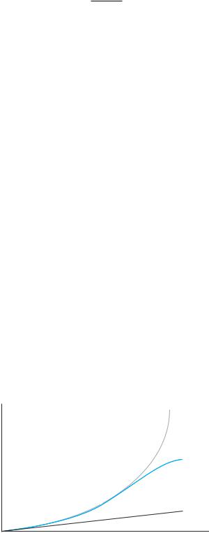
The best mathematical model for the shape of the species-area curve has been debated over the years. Three candidates have been proposed: the exponential curve,

S = Z ln(A) + C

the power curve,

S = CAZ

and the logistic curve,

S = B

C + A−Z

where S is the number of species, A is the area, and B, C, and Z are constants (Figure 12.4). The three equations are actually members of the same mathematical family,

PAGE PROOF: 2ND PASS

such that the exponential function is a special case of the power function—that is, they are equivalent when

C

= Z ln( A)

AZ − 1

and the power function, in turn, is a special case of the logistic function—that is, the power and logistic functions are equivalent when

Which of the three curves best fits a given data set? This depends on the area being sampled and the scale of environmental variation. For small or intermediate-sized areas, a logistic curve often fits bests, while for large areas a power curve is often the best fit.

These three models make different assumptions about the relationship of species number to area. Both the exponential and power functions result in curves that continue to rise indefinitely. The logistic function, on the other hand, eventually reaches a plateau. This distinction is important if one wishes to answer the question, “How many species are in the community?” If the species-area curve rises indefinitely with increasing area, then the answer depends entirely on the area of the community. However, the “area” of a community is often arbitrary, making the question meaningless. Instead, we can rephrase the question as, “How many species are contained in an area of size X?” This value is known as species density. If the species-area relationship is best described with a logistic curve, then this question has meaning, because the curve has a definite plateau or asymptote, calculated as B/C. The issue of the shape of the species-area curve will become important when we explore comparisons of diversity among communities in Chapter 16.

ln (Area)

Figure 12.4

Examples of three differently shaped species-area curves: exponential, power, and logistic.

Community Properties 241

An alternative method of estimating species richness is to ask how many species are found in a sample of some number of individuals. For some functional groups, such as trees, in which individuals are easy to identify, this approach can be useful. Mathematical techniques, called rarefaction, exist for standardizing estimates among samples that include different numbers of individuals and for estimating the number of very rare species that were missed in the sample (Krebs 1989). These techniques were developed first and are used most often in animal ecology, although they are being used increasingly by plant ecologists. Because animals often move, area-based measures are less useful to animal ecologists. Plant ecologists, on the other hand, tend to emphasize area-based techniques because the clonal nature of many plants can make it difficult to distinguish individuals (see Chapter 8). In plant ecology, dry weight (the weight of a sample after it has lost all its moisture and is at a constant weight), or biomass, is often used instead of number of individuals.

How is the number of species in a community actually determined? One can use species-area curves to determine the total area required for standardized sampling. By using equal areas in different stands within a particular community, we avoid differences due to sampling intensity. We may also wish to compare different community types in a study using the same methods. For example, we might sample a beech-maple community and an oak-hickory community using the same approach. For very different kinds of plant communities, however, such as grasslands and forests, we might need to use different sampling areas and somewhat different techniques to best determine the characteristics of each.

How large an area should be sampled? We want a sample that is large enough to contain most of the species and which will minimize differences due to random sampling effects, such as where plots happen to be placed. On the other hand, for practical purposes, we do not want the area to be bigger than necessary. With respect to a species-area curve, we want to sample a total area for a given community that is at least as large as the point at which the curve begins to level off at a plateau, or, if there is no plateau, at which the rate of increase with increasing area is very small. We will return to the particular methods used for sampling vegetation shortly.

Diversity, Evenness, and Dominance

Species richness is only one aspect of diversity. Not all species exist in equal numbers: some are rare, some are common but not numerous, and others are very abundant. Imagine two forest stands, both of which contain a total of 100 individuals (or 100 kg of biomass) belonging to 5 different species. In one forest stand, there are 20 individuals of each species. In the other, one species has 60 individuals, while each of the other 4 species has