Jessica Gurevitch, Samuel M. Scheiner, and Gordon A. Fox - The Ecology of Plants - 2002 / The Ecology of Plants Jessica Gurevitch, Samuel M. Scheiner, and Gordon A. Fox; 2002 / Ch 06

102 Chapter 6

In the last chapter we described how natural selection works. In this chapter we explore examples of the results of natural selection and the process of speciation. The examples in this chapter were chosen because they are based on more than just speculation. Most of them are based on multiple lines of evidence. As we examine each, we discuss the reasoning behind the conclusions concerning the shaping of the trait by natural selection.

This brings us back to the question we posed in the first sentence of this chapter: Why is it so difficult to decide whether a trait was shaped by natural selection? While natural selection is a primary process in shaping plant form and function, other processes may also be responsible for shaping particular traits. In some instances these processes act in concert with natural selection. Mammals have backbones not only because a backbone is a handy thing to have, but because they are vertebrates, and they have inherited this trait from vertebrate ancestors: all vertebrates share this trait for that reason. Likewise, angiosperm cells exhibit cellular respiration not because it is especially advantageous to angiosperms per se, but because the ancestors of angiosperms possessed this trait, which they have inherited, and thus share with a much broader group of living organisms.

In addition, natural selection is only one of the factors that cause evolutionary change (see Chapter 5). Other processes may act in concert with natural selection, or they may act against it, or they may act independently. Mutation, for example, is a necessary source of the variation that natural selection requires. Migration of individuals from other environments can prevent adaptation to local conditions in response to natural selection. Genetic drift can also cause changes in gene frequencies. Often each of these three processes can produce results that look like the outcome of natural selection. Because we are reconstructing a historical event, our conclusions must be based on indirect inference, rather than direct observation. All of these factors make the determination of adaptation by natural selection a challenging task.

Heavy-Metal Tolerance

We begin with one of the best-documented cases of natural selection and local adaptation in plants. This example is also important historically: it was the first demonstration of fine-scale genetic differentiation in response to selection by a known factor in the environment. The example involves a cline, a gradient in genetic composition, resulting from genetic differentiation and adaptation. Clines can occur over very short distances as well as over larger geographic scales.

In the 1960s, A. D. Bradshaw and his students (e.g., Jain and Bradshaw 1966; McNeilly and Antonovics 1968;

PAGE PROOF: 2ND PASS

Antonovics and Bradshaw 1970) began to study local adaptation of grasses to differ-

ences in soil conditions due to mine waste contamination. In Great Britain, zinc and copper have been mined for centuries. The soil left over from the diggings and ore extraction, known as tailings, was simply dumped outside the mines. Although most of the ore had been removed, these tailings still contained high concentrations of the metals, concentrations too low to be worth

extracting but still high enough to be toxic to most plants growing on the soil. Some plants, however, managed to grow on these tailings—in particular, the grasses

Anthoxanthum odoratum and Agrostis tenuis. Although some of the mines had been abandoned for only a cen- tury—probably fewer than 40 generations for these perennial species—the researchers found that populations of these grasses on the mine tailings were tolerant of the heavy metals, while plants growing in ordinary adjacent pastures were not. The tolerance of heavy metals was achieved by the evolution of biochemical mechanisms that prevented the uptake of the toxic ions. These differences in genetic composition occurred over very short distances—within a meter of the mine boundary (Figure 6.1).

The abrupt nature of the genetic boundary illustrates several aspects of the evolutionary process. First, the alleles for heavy-metal tolerance did not spread outward from the population on the mine tailings. Why? Experiments were performed in a greenhouse in which plants from both the mine tailings and the adjacent pasture were grown in soil with and without the heavymetal contaminants. As expected, plants from the pasture population died when grown with the heavy metals, usually as seedlings. However, when grown in the absence of the heavy metals, the pasture plants grew much more quickly than those from the mine tailings population. Something about the mechanism of tolerance reduced growth under uncontaminated conditions. This interaction is an example of a trade-off, a reduction in fitness in one feature of an organism due to an increase in fitness in another feature. In this case, heavymetal tolerance and growth in uncontaminated soils are traded off against each other. Thus, different alleles are favored on and off the mine tailings, and the populations have diverged genetically due to natural selection.

Other features of the populations have also evolved as a consequence of this divergence. All grasses are wind pollinated, so pollen from the adjacent pastures can easily land on the stigmas of plants on the mine tailings, and vice versa. The abruptness of the genetic boundary was

PAGE PROOF: 2ND PASS

Distance (m)

Figure 6.1

Ability of adults and plants grown from seeds of Agrostis tenuis collected from mine tailings and from adjacent uncontaminated pasture to grow in the presence of copper. Some 100 years after the mine was abandoned, the genetic composition of the grass population differs dramatically at the mine boundary, where alleles for enzymes that prevent the uptake of toxic ions are suddenly favored. (After McNeilly 1968.)

found to be related to the prevailing wind direction, with more of the “wrong” genotype being found on the downwind side. If an individual is pollinated by a plant from the other population, then its offspring will be less well adapted to the local conditions, as shown by the lower tolerance of the plants grown from seed in Figure 6.1. The problem of “wrong” pollinations results in selection for mechanisms that reduce cross-pollination. In these populations, two mechanism were involved in reducing outcrossing (Antonovics 1968; McNeilly and Antonovics 1968). First, individuals on the mine tailings tended to flower earlier than those in the pasture, with the difference being greatest for plants just at the boundary of the mine tailings. Second, plants near the boundary tended to self-pollinate more than plants farther away from the boundary. Both changes reduced the chance of an individual receiving the “wrong” pollen from plants adapted to the alternate conditions (toxic or uncontaminated soils). These changes in mating patterns were a secondary consequence of the primary selection for heavy-metal tolerance. They acted to reinforce the genetic differentiation of the populations. Over a long enough period of time, such reinforcement can lead to total genetic isolation of the populations, and ultimately to speciation.

Outcomes of Evolution 103

These studies clearly demonstrate, for several reasons, that the differences among populations were due to natural selection. First, the investigators demonstrated the presence of all three necessary components of natural selection: phenotypic variation, fitness differences, and heritability (see Chapter 5). Second, they found that secondary predictions were also met. The change in flowering time, for example, was a consequence of natural selection for heavy-metal tolerance. Third, they found the pattern of adaptation repeated both among populations of the same species at different mines and among different species. Such repeated patterns of differentiation would be very unlikely to have occurred by chance alone. For all of these reasons, we conclude that the differences in heavy-metal tolerance between populations on and off the mine tailings were due to evolution by natural selection.

Ecotypes

Plant ecologists and taxonomists have recognized since before the time of Linnaeus, well over 250 years ago, that the same kind of plant may have a different appearance depending on where it is growing. Early in the twentieth century, researchers in Europe and in the United States began careful experimental work to better understand the causes of some of these differences. In Sweden, Turesson (1922) collected plants belonging to several dozen species from habitats all over Europe and grew them in a common garden experiment at a single site in Sweden. He found that many of the differences that he noticed when the plants were growing in their natural habitats were retained when they were all grown in a single environment. Turesson coined the term ecotypes to describe populations of a species from different habitats or locations that possess genetically based differences in appearance and function. Ecologists usually use the term “ecotype” to refer to such differences that appear to be adaptive.

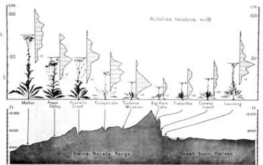
At about the same time as Turesson was doing his experiments in Sweden, Clausen, Keck, and Hiesey (1940) were doing similar work in California. These researchers established three common garden sites at low, intermediate, and high altitudes, from the Carnegie Institute south of San Francisco, where they worked, up into the high Sierra (the spectacular Sierra Nevada that John Muir, the famous conservationist, called “the range of light”). Plants from a large number of species were collected along a transect—a long line along which samples are taken—running from the coast of California inland, up to the highest part of the Sierra Nevada and down the arid eastern side of the mountains (Figure 6.2). The plants were vegetatively propagated, and genetically identical copies of many different individual plants were grown in each of the three gardens. Clausen, Keck, and Hiesey

104 Chapter 6

PAGE PROOF: 2ND PASS

studied two groups of species most intensively: several closely related species of Achillea (yarrow, Asteraceae), and Potentilla glandulosa (cinquefoil, Rosaceae).

Like Turesson, the researchers found that many of the differences in morphology (growth form) and phenology (the timing of seasonal events, such as flowering and dormancy) among plants from different sites were still present when those plants were compared in the common gardens (Figure 6.3). Achillea plants from lower sites were larger than plants from higher altitudes, with longer leaves and taller flower stalks. Plants from higher altitudes generally entered dormancy sooner and began growing later than plants from lower, warmer sites. These alpine (high-mountain) plants also tended to flower later than those from lower-altitude sites. Plants generally had the highest survival rate and best performance in the garden with the conditions that most closely resembled those in which they grew naturally (Clausen et al. 1948). The researchers also noted striking differences in the appearance of the leaves from different sites along the transect. Leaves from the high-altitude populations were not only smaller, but tended to have a dense gray pubescence (a mat of short hairs on the leaf surface), and were much more compact in shape. Leaves

from lower-altitude plants were smooth and green, and were highly dissected (had a blade divided into small but connected parts, making the leaf look very feathery).

Many years after these original studies, Gurevitch and colleagues (Gurevitch 1988, 1992a,b; Gurevitch and Schuepp 1990) returned to the original sites to carry out further studies on the same populations that Clausen, Keck, and Hiesey had worked on. As anyone who has visited or lived in California might expect, sadly, many of the original sites where plants had been collected are now under asphalt. However, the Carnegie Institute still maintains the sites at Mather and Timberline, where two of the common gardens once were located, and plants from these intermediateand high-altitude populations were collected for study. The populations differed genetically in photosynthetic characteristics. There were also genetic differences between the populations in both leaf size and leaf shape, particularly in the degree to which these complex leaves were dissected. As the early researchers had noticed, the Mather population had much more feathery, highly dissected leaves, while those from the Timberline plants were more compact (Figure 6.4).

Could there be an adaptive reason for these differences in leaf shape? Energy budget studies demonstrat-

PAGE PROOF: 2ND PASS

Figure 6.3

Appearances of 7 clones from the Mather population of Achillea lanulosa (collected at 1400 m. elevation) when grown in the three transplant gardens. Timberline (top; 2100 m.), Mather (center), and Stanford (bottom; 30 m. elevation). (From Clausen et al. 1948.)

ed that the highly dissected leaves of the Mather plants had a thinner boundary layer with greater heat conductance (see Chapter 3), making it more likely that they would remain close to air temperature. The compact leaves of the high-altitude plants had a thicker boundary layer and less heat conductance, and energy budget calculations suggested that these leaves could warm considerably above air temperatures. Thus, in the warm,

Outcomes of Evolution 105

dry environment at the lower altitude, leaves would remain relatively cool, while high-altitude plants might be able to warm up above the chilly air temperatures common in their environment to maximize photosynthesis and growth.

Another study taking a similar approach was carried out on the widespread European species Geranium sanguineum (Geraniaceae; Lewis 1969, 1970). This species grows in a variety of habitats. As Turesson himself and other researchers had noticed for other species, plants of this species from the most xeric (dry) sites had the most highly dissected leaves, with the narrowest lobes, while those from more mesic sites (with more water available) had larger, less dissected leaves (Figure 6.5). Lewis found genetic differences in leaf shape and size among plants collected from a large number of different sites in Europe. There was a cline in the degree of leaf dissection, with the most highly dissected leaves from the driest environments and the more compact leaves from moister, more oceanic sites. A different geographic cline in leaf size correlated with the openness of the habitat, with the largest-leaved plants from the least open, most tree-shaded habitats. Based on physiological and energy budget studies, he hypothesized that differences in leaf energy budgets due to the differences in leaf size and shape would lead to differences in leaf temperatures. The more dissected leaves from the drier habitats would remain closer to air temperature, thus potentially avoiding overheating when drought forces stomatal closure. Other physiological advantages were also predicted for leaves of each ecotype in its “home” environment.

Originally, it was believed that there was a strict dichotomy between clines and ecotypes. Clines represented gradual differences in genetic characters, responsible for gradual morphological and physiological differences over geographic space. Ecotypes, in contrast, represented sharp differences among populations that are distinct genetically and in various phenological traits. Most plant ecologists no longer see this distinction as being very useful. Genetic variation responsible for morphological, physiological, and phenological differences may occur over many different scales, sometimes with sharp distinctions among populations and sometimes with gradual change. The abruptness of the change depends on the nature of the evolutionary processes acting on these groups of plants: selection, genetic drift, and migration all shape the rate of genetic change over space. We may choose to call distinctive populations “ecotypes” for convenience, or we may wish to emphasize the gradual nature of change and call the gradient a “cline.” As natural habitats grow ever smaller and more fragmented, more and more cases of gradual genetic and phenotypic change in plant and animal populations will become isolated, thus resembling ecotypes even though their origins were as members of a continuously varying cline.

106 Chapter 6

PAGE PROOF: 2ND PASS

5 cm

Dry, open

Adaptive Plasticity

For the most part, plants are not mobile. This observation, while obvious, has profound implications for the evolution

and adaptation of plants. If the environment becomes unfavorable in one spot, a mobile animal can move to a more favorable location. But what can a plant do?

Because plants cannot move, they must be able to tolerate environmental variation. As discussed in Chapter 5, one solution to this problem is for individuals to be phenotypically plastic, able to change their form so as to match the most fit trait value for the environment they find themselves in (Bradshaw 1965). For example, plants produce leaves with different characteristics when grown in the sun than when grown in the shade (see Chapter 2). Plants in general are far more plastic than animals; for example, while well-fed animals are taller and heavier than those with poorer diets, plants grown under optimal conditions can be orders of magnitude larger than genetically identical plants grown in poor conditions.

Moist, shaded

But how do we demonstrate that plasticity itself is adaptive, or investigate the conditions under which it is most advantageous? Many characteristics of plants vary with the environment. While some of this variation is adaptive, some changes in plant appearance and function are merely unavoidable consequences of

PAGE PROOF: 2ND PASS

Figure 6.6

Impatiens capensis (Balsaminaceae) grown in the sun (high red:far-red ratio) and in the shade (low red:far-red ratio). Short, stout plants are favored in low-density conditions, while tall, thin plants are favored in crowded conditions. (Photograph courtesy of J. Schmitt.)

plant physiology, such as having yellow leaves when deprived of sufficient nitrogen. Demonstrating that phenotypic plasticity is adaptive requires, first, that there be more than one possible response, and second, that there is a consistent relationship between plasticity and fitness. The following study demonstrates how one can amass evidence on these points.

Johanna Schmitt and her colleagues studied populations of Impatiens capensis (jewelweed, Balsaminaceae) growing in different light conditions (Schmitt 1993; Dudley and Schmitt 1995, 1996). This species is an annual that grows in deciduous forests of the northeastern and north-central United States. Jewelweeds grow in conditions from full sun to forest understories, often along streams, and can reach very high densities.

A typical response to crowding in plants is stem elongation. This strategy allows a plant to overtop its close neighbors, thus gaining the most light (Figure 6.6). In uncrowded situations, however, plants remain short, because elongation has costs as well as advantages. More resources must be put into support structures rather than flowers and seeds, and the elongated stem is thinner and in greater danger of falling over. The elongation response is controlled by the ratio of red to far-red light that a plant receives (see Chapter 5).

Is it possible that a plant can tell whether or not it is growing near other plants, and thus at risk of even-

Outcomes of Evolution 107

tually becoming shaded by its neighbors? If so, a plant finding itself in this situation will benefit by elongating its stem as it grows. If it can detect the fact that it is growing in an uncrowded environment, it may be better off not elongating its stem very much. The chlorophyll in the leaves of neighboring plants absorbs heavily in the red part of the spectrum. Therefore, a plant that receives light with a low red:far-red ratio can use that information as a signal that it is surrounded by other plants.

Is the elongation response truly adaptive? Schmitt addressed this question by manipulating plant form and growing conditions. Seedlings were initially grown in a greenhouse under two conditions: (1) with filters that blocked the red part of the light spectrum and (2) with full-spectrum controls that reduced light by the same amount without changing the red:far-red ratio. These treatments created two sets of plants, elongated and suppressed. The experimental plants were then transplanted into a forest at either high or low density. Fitness was measured as the total number of seed capsules present at the end of the summer. As predicted by the adaptive plasticity hypothesis, the elongated form had higher fitness under crowded conditions, while the short, stout form had higher fitness at low densities (Figure 6.7).

The pattern of plasticity also differed in an adaptive way among populations growing in different environments. The researchers compared three populations

Density

Figure 6.7

A test of adaptive plasticity of stem elongation in Impatiens capensis. Elongated plants were initially grown in a greenhouse with filters that blocked the red part of the light spectrum; suppressed plants were grown with full-spectrum controls that reduced light by the same amount without changing the red:far-red ratio. The two sets of plants were then grown at high or low density. The bars indicate 1 standard error. (After Dudley and Schmitt 1996.)

108 Chapter 6

growing within 1 kilometer of one another, one in a woodland clearing and the other two in the woods. They grew plants from all three populations together in a greenhouse. The clearing population had a stronger elongation response than the other two populations. This result is predicted on adaptive grounds: In the woods, a plant that grows taller than its neighbors will still be in the shade. On the other hand, in a sunny site, a plant that overtops its neighbors will be in bright light. Thus, being more plastic is adaptive for the population in the clearing. As in our first example, here again the researchers showed the existence of the three necessary components of natural selection: plants varied in how plastic they were, differences in plasticity led to fitness differences, and plasticity was shown to be heritable. Finally, they showed that differences in plasticity among populations were in the direction expected if plasticity were evolving by natural selection.

The term “plasticity” is used in two different contexts by ecologists. We have already discussed one context, the plasticity of an individual. The other context is the plasticity of a species, meaning the range of ecological conditions that a species will grow in. This range is also called the species’ niche (Grinnell 1917). The niche of a species is determined by the sum of the niches of its members (Figure 6.8). Those individuals may be plastic and may have wide or narrow niches. They may vary genetically in their optima. If they vary sufficiently, they may be referred to as ecotypes. So, a species may consist of a combination of generalist and specialist genotypes, while at the same time we speak of generalist and specialist species. In plant ecology, the idea that the total

Survival probability (%)

0

Figure 6.8

The niche of a species is the sum of the niches of its members. Here we consider one aspect of a niche, temperature tolerance. In this graph, each solid curve is the survival probability of an individual as a function of temperature. The temperature range of the curve is one measure of plasticity of that individual. The dashed curve is, then, the niche of the species.

PAGE PROOF: 2ND PASS

variation in a species can result from some combination of plastic and nonplastic genotypes traces to an influential paper by Bradshaw (1965). However, only in the past 20 years has this distinction begun to be more widely recognized (see reviews by Schlichting 1986; Sultan 1987; West-Eberhard 1989; Scheiner 1993; Via et al. 1995; Pigliucci 2001).

We also speak of two versions of the niche, the fundamental niche and the realized niche (Hutchinson 1957). The fundamental niche is the range of conditions that a species is physiologically capable of growing in. The realized niche is the range it is actually found in. Factors such as competition, herbivory, and lack of pollinators or seed dispersers all act to reduce a species’ realized niche from the potential of its fundamental niche; these factors will be covered in more detail in Chapters 8 through 11, and Leibold (1995) offers a comprehensive review of niche concepts.

Selection in Structured Populations

The fitness of an individual depends on its environment. One component of that environment is population structure: the phenotypes of the other individuals in the population and their frequencies. In Chapter 7 we describe two types of population structure, age structure and stage structure, but there are also other sources of phenotypic variation among the individuals in a population, such as the colors or shapes of their flowers. When the fitness of an individual depends on the number and kinds of other phenotypes in the population, selection can take various forms. Two of these forms are frequen- cy-dependent selection and group selection; here we explore examples of both types.

Frequency-Dependent Selection

Frequency-dependent selection occurs when the fitness of a genotype depends on whether it is common or rare in a population. An example is seen in the evolution of mating systems in Lythrum salicaria (purple loosestrife, Lythraceae; see Figure 14.3). This species is an invasive weed in wetlands of northern North America. It is still in the process of invading the continent, which makes it an ideal species for studying evolution in action. In the study described here, scientists were able to directly observe populations evolving over a five-year period.

Lythrum salicaria has an unusual mating system, called tristyly. The style is the female reproductive structure that supports the stigma, upon which pollen lands to fertilize the ovules (see Figure 8.6). This mating system gets its name because individual plants in a population have one of three different forms for the style: short, medium, or long (Figure 6.9A). The form of the style is genetically determined. The style lengths are matched by three stamen lengths (the stamen supports

PAGE PROOF: 2ND PASS

Morph 2 (medium style)

Morph 3

Lythrum salicaria (short style) (purple loosestrife)

Figure 6.9

(A) Tristyly in purple loosestrife (Lythrum salicaria, Lythraceae). The plant has three different forms, or morphs, of stamen and style, a system that promotes outcrossing. An individual with a given style length can mate only with the other two stamen types. (B) Change in style length evenness over a five-year period in 24 populations of L. salicaria. An evenness value of 1 would indicate that the three lengths were equally frequent. In all but 4 of the populations, the frequencies were more even in year 5 than in year 1, indicating that the rare morph had increased in frequency. (B after Eckert et al. 1996.)

the anthers, which hold the pollen). A single individual has a style of one length and stamens of the other two lengths. This system is a way of enforcing outcrossing. An individual with one style length cannot mate with another individual with the same style length; it can mate only with the other two types. (See Chapter 8 for more details on mating systems and tristyly.)

Frequency-dependent selection comes about because of this inability to mate with other individuals of the same type. Imagine a population of 99 long-styled individuals and 1 individual with short styles. That short-styled individual would be able to mate with all the other plants, as it could fertilize all the other plants in the population with its pollen. The long-styled plants would be limited to pollinating just the one short-styled individual. So in the next generation, the genes of the short-styled individual would end up in the offspring of 100 plants (itself through its female gametes and the

Outcomes of Evolution 109

(B)

other 99 plants through its pollen). In contrast, each of the long-styled individuals would have offspring through at most 2 plants (themselves and the shortstyled plant). As a result, the genes of the short-styled plant would increase in frequency. In general, the rarest mating type (the one with the least common style length) will always enjoy this sort of mating advantage. The population will therefore continue to evolve until all three types are at equal frequency, with one-third of the population having each of the style types.

Just such a pattern of evolutionary change was observed by Christopher Eckert and colleagues (1996), who surveyed 24 populations of L. salicaria across the Canadian province of Ontario. These populations were newly established as part of the invasion of L. salicaria into North America. During the creation of each population, some style length types had a high frequency while others had a low frequency due to chance alone. Sometimes it was the short type that was rare, sometimes it was the medium type, and sometimes it was the long type. The researchers predicted that over time the populations should evolve to an equal frequency of the three types. They tested this prediction by returning to the populations 5 years later. The prediction was met: In all cases, the rarest style length had increased in frequency (Figure 6.9B). Most of the populations were still not yet at equilibrium, with one-third of each type; that will require several more decades. However, the populations had consistently evolved in the predicted direction, something that would be highly unlikely to occur by chance.

110 Chapter 6

PAGE PROOF: 2ND PASS

This example is an instance in which natural selection is strong enough that we can observe its effects in action. It is unusual to be able to measure a consistent change in a natural population in just 5 years. Part of the strength of this study is that this change was observed across 24 different populations. Thus, it is highly unlikely that the change is due to anything other than natural selection. So, we can be confident that what we are observing is evolution by natural selection.

Group Selection

Group selection occurs when variation in group characteristics causes differences in fitness among groups. We briefly described the basis of group selection in Chapter 5 in the discussion of levels of selection. Group selection is one term used for selection above the level of the individual. A common form of group selection is kin selection, which occurs when the groups in question consist of closely related individuals.

The concept of group selection is somewhat controversial among evolutionary biologists. Kin selection is less controversial because the individuals in a group are closely related, and thus share large numbers of genes. No one disputes that group characteristics can affect individuals’ fitness. However, group selection also implies that group-level characteristics can be subject to natural selection. Whether selection on group-level traits has occurred outside of kin groups is a matter of dispute.

An example of group-dependent fitness effects was found in populations of Impatiens capensis (Stevens et al. 1995). These plants often grow in dense patches, or groups of plants, as we saw in Schmitt’s work on adaptive plasticity. Impatiens can produce both closed, selfpollinated flowers (cleistogamous flowers) and open, potentially cross-pollinated flowers (chasmogamous flowers) on the same plant. In this study, plant size and fitness were measured; fitness was measured as the number of either cleistogamous or chasmogamous flowers produced on each plant by the end of the growing season. The researchers then compared the flower production among groups (patches). Some patches had mostly small individuals, and thus a small mean plant size. Other patches had a few large individuals surrounded by small neighbors; in these patches the average plant size was large, due to the very large size of the dominant individuals. Both individual-level and grouplevel selection was found (Figure 6.10). Individual-level selection occurred within each patch, because larger individuals within a patch had greater numbers of both kinds of flowers. Group-level selection occurred among patches, because individuals in patches with a small mean plant size produced, on average, greater numbers of closed flowers than did individuals in patches with a large mean plant size. (There was no group-level selection on the number of open flowers.) That is, the char-

Figure 6.10

Individualand group-level selection on size in Impatiens capensis. Fitness was measured as the number of cleistogamous flowers (A) and chasmogamous flowers (B) produced. The black lines show the relationship between an individual’s flower production and the individual’s size—a result of individual-level selection. The green lines show the relationship between an individual’s flower production and the average size of the other individuals in its patch—a result of group-level selection. (After Stevens et al. 1995.)

acteristics of the group determined the number of flowers, and thus the fitness of individuals.

How could this occur? Individuals with small neighbors had greater numbers of cleistogamous flowers than those with large neighbors. In patches where the mean size of individuals was large, only the largest individuals were able to produce cleistogamous flowers. These very large individuals depressed the flower production of their smaller neighbors by shading them and reducing their access to resources. Yet the large individuals did not completely use up the resources in the patch; some resources went unused. In contrast, in patches where the mean size of individuals was small,