

PAGE PROOF: 2ND PASS
P A R T |
II |
Evolution and |
|
|
|||
|
Population Biology |
||
|
|
||
|
|
|
|
|
|
5. |
Processes of Evolution 87 |
|
|
6. |
Outcomes of Evolution 101 |
|
|
7. |
Population Structure, Growth and Decline 117 |
|
|
8. |
Growth and Reproduction of Individuals 143 |
|
|
9. |
Life Histories 167 |
|
|
|
|
PAGE PROOF: 2ND PASS
PAGE PROOF: 2ND PASS
C H A P T E R 5 Processes of Evolution
In Part I, as we explored the various ways in which plants interact with their environments, we looked at the features of plants that permit them to cope with different environments. All of those features arose through the process of evolution by natural selection. The most amazing aspect of this process is how a few simple consequences of biology and natural laws have resulted in the vast diversity of life. All of the species that compose ecological communities arose through evolution, and ecological processes provide the context for evolution. The ecologist G. Evelyn Hutchinson emphasized this intimate relationship in his seminal book, The Ecological Theater and the Evolutionary Play (1965). The intertwining of evolution and ecology is greatest in the process of natural
selection.
This chapter and the next summarize the basic principles and processes of evolution and explore its outcomes. In this chapter, we cover the process of natural selection as well as other processes that affect evolution. In Chapter 6, we examine a series of specific examples of evolution by natural selection.
Natural Selection
Natural selection occurs when individuals with differing traits leave different numbers of descendants because of those differences. Evolution by natural selection occurs when those differences are heritable (have a genetic basis). Adaptive traits are ones that have come about through the process of evolution by natural selection. The suite of traits associated with CAM photosynthesis (see Chapter 2), for example, is adaptive in hot, dry climates because individuals that have those traits are able to leave more descendants than individuals that do not. Arctic plants are short-statured because by remaining close to the ground they remain warmer, grow more, and ultimately leave more offspring.
The principles of natural selection were first proposed by Charles Darwin in his book On the Origin of Species by Means of Natural Selection, published in 1859. Natural selection is one of the four central processes of evolution. The others are mutation, migration, and genetic drift.
Variation and Natural Selection
An important starting point for any discussion of evolution and natural selection is variation. Variation is ubiquitous in nature. Nearly all natural phenomena vary
88 Chapter 5
at some level. This principle is expressed in the adage that “no two snowflakes are exactly alike.” Living beings are much more complex than snowflakes, with an even greater potential for different kinds and amounts of variation. Evolution requires two kinds of variation: phenotypic variation and genetic variation.
Plants, like most living organisms, vary phenotypically. The term phenotype refers to all of the physical attributes of an organism. These properties include aspects of outward appearance (such as height, leaf size and shape, flower color, or fruit number), behaviors (such as growth of roots toward water), life history characteristics (such as being an annual), internal anatomy, and the content of cells (such as protein composition).
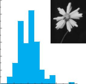
Phenotypic variation can be extensive for traits such as seed size, which can vary 20-fold within a single population of a wildflower species (Figure 5.1), or biomass, which can vary over several orders of magnitude in trees. Other kinds of traits, such as flower size and solute concentrations in cells, tend to vary much less among individuals in a population. Still other traits, such as petal number or photosynthetic pathway, tend to be invariant within a species. However, even these traits vary within some species (see Chapter 2). Furthermore, the particular pattern of growth and development exhibited by an individual plant depends on a complex interaction between its genes and its environment. All of these differences among individuals result in phenotypic variation.
|
30 |
|
|
|
|
|
sampleof |
25 |
|
|
|
|
|
20 |
|
|
|
|
|
|
Percentage |
|
|
|
|
|
|
15 |
|
|
|
|
|
|
|
|
|
|
|
|
|
|
|
|
|
|
Coreopsis lanceolata |
|
|
10 |
|
|
|
|
|
|
5 |
|
|
|
|
|
|
0 |
|
|
|
1.6 |
|
|
0.0 |
0.4 |
0.8 |
1.2 |
2.0 |
|
|
|
|
Seed mass (mg) |
|
|
|
Figure 5.1 Variation in individual seed mass in a population of Coreopsis lanceolata (Asteraceae) growing on an inland dune south of Lake Michigan. (Data from Banovetz and Scheiner 1994.)
PAGE PROOF: 2ND PASS
The genotype of an individual is the information contained in its genome—the sequence of its DNA. This information is expressed through the processes of transcription of DNA to RNA and translation of the RNA into protein. Gene expression, and the development of the plant as a whole, is controlled by the information contained within the genome itself through various feedback mechanisms. A seed contains all of the information necessary for the growth and development of the adult plant. Development can be thought of as the unfolding of the information contained in the genome.
The Components of Natural Selection
Natural selection requires three components: phenotypic variation among individuals in some trait; fitness differences (some individuals must leave more descendants than others as a result of the phenotypic differences), and heritability (the phenotypic differences must have a genetic basis). If these three components are present for a trait within a population, then the frequency of that trait will change in that population from one generation to the next: evolution by natural selection will occur.
Fitness differences include differences in mating ability, fecundity (number of gametes produced), fertilizing ability, fertility (number of offspring produced), and survivorship (chance of surviving). What causes these fitness differences? It could be chance. But often these differences are associated with differences in some trait of the plants. Phenotypic selection occurs when individuals with different trait values have consistent differences in fitness.
A useful and convenient way to study the process of natural selection is to subdivide it into two parts: that which occurs within a single generation—phenotypic selection—and that which occurs from one generation to the next—the genetic response (Endler 1986). Phenotypic selection consists of the combination of phenotypic variation and fitness differences. This part is what we often think of as natural selection. But for evolution to occur, the other part—the genetic response—is equally important. The genetic response is the change in the genetic makeup of the population that occurs from one generation to the next. The genetic response depends on the heritability of a trait. If a trait is heritable, then if phenotypic selection favors that trait in one generation, the next generation will have a greater proportion of individuals with that trait.
In a population of the grass Danthonia spicata, for example, individuals with longer leaves had higher survivorship and fecundity than individuals with shorter leaves (Figure 5.2A). Variation in leaf length is known to be at least partially under genetic control. So the next generation, on average, will be likely to have longer leaves. From one generation to the next, the change in the population may be small. But if the process of natu-
PAGE PROOF: 2ND PASS
Processes of Evolution 89
(A) |
|
|
|
|
|
|
(B) |
|
|
|
|
|
|
5 |
|
|
|
|
|
|
6 |
|
|
|
|
|
4 |
|
|
|
|
|
|
5 |
|
|
|
|
|
|
|
|
|
|
|
|
|
|
|
|
|
|
3 |
|
|
|
|
|
|
|
|
|
|
|
fitness |
2 |
|
|
|
|
|
fitness |
4 |
|
|
|
|
|
|
|
|
|
|
|
|
|
|
|||
|
|
|
|
|
|
|
|
|
|
|
|
|
Relative |
1 |
|
|
|
|
|
Relative |
3 |
|
|
|
|
0 |
|
|
|
|
|
2 |
|
|
|
|
||
|
|
|
|
|
|
|
|
|
|
|
||
|
|
|
|
|
|
|
|
|
|
|
|
|
|
–1 |
|
|
|
|
|
|
|
|
|
|
|
|
–2 |
|
|
|
|
|
|
1 |
|
|
|
|
|
|
|
|
|
|
|
|
|
|
|
|
|
|
–3 0 |
4 |
8 |
12 |
16 |
20 |
|
0–4 |
–2 |
0 |
2 |
4 |
|
|
|
Leaf length (cm) |
|
|
|
|
|
Late growth rate |
|
|
|
(C)
Relative fitness
|
|
|
(D) |
|
|
|
|
5 |
|
|
|
4 |
|
|
|
4 |
|
|
fitness |
3 |
|
|
|
3 |
|
|
Relative |
2 |
|
|
|
|
|
|
|
|
|
||
2 |
|
|
|
1 |
|
|
|
|
|
|
|
|
|
|
|
1 |
|
|
|
100 |
|
|
|
|
|
|
|
80 |
|
|
|
0 |
|
|
|
60 |
|
|
8 |
|
|
Water use |
40 |
|
6 |
||
|
|
|
|
4 |
|||
|
|
|
efficiency |
20 |
2 |
||
|
|
|
Leaf length (cm) |
||||
–1 |
|
|
|
|
0 |
||
1 |
2 |
3 |
|
|
0 |
|
|
0 |
|
|
|
|
|||
Corn earworm damage
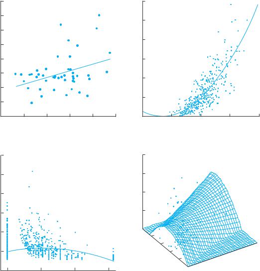
Figure 5.2 Relationships between phenotypic variation in plant traits and fitness differences result in phenotypic selection. If genetic variation for these traits also exists, then evolutionary change may occur. (A) Directional selection for longer leaf length in the perennial Danthonia spicata (poverty grass, Poaceae) in a natural population growing in a white pinered oak forest in northern lower Michigan. Fitness was measured as the total number of spikelets produced over five years and was corrected for correlations with other traits. (Data from Scheiner 1989.) (B) Directional selection for greater growth rate late in the season in the annual Impatiens capensis (jewelweed, Balsaminaceae) in a natural population growing in a deciduous forest in Wisconsin. Fitness was measured as the final dry weight of the plant, which is correlated with the number of seeds produced. The fitness function is curved, but still monotonically increasing. (After Mitchell-Olds and Bergelson 1990.) (C) Stabilizing selection for the amount of damage caused by the corn earworm to the annual Ipomoea purpurea (morning glory, Convolvulaceae) in an experimental population growing in an old field in North Carolina. Fitness was measured as the number of seeds produced by the end of the growing season. (Data from Simms 1990.) (D) Stabilizing selection for water use efficiency and directional selection for smaller leaf size in the annual Cakile endentula (sea-rocket, Brassicaceae) in an experimental population growing on a beach along southern Lake Michigan. Fitness was measured as the number of fruits produced by the end of the growing season. The optimal water use efficiency depends on leaf size, which is an example of correlational selection. (After Dudley 1996.)
90 Chapter 5
ral selection goes on for many generations, the population may become very different from its ancestor. Much of the striking variation among species is due to such long-term evolutionary responses to natural selection.
Directional selection occurs when individuals with the most extreme value for a trait have the highest fitness (Figure 5.2A,B). In this case, the population will continue to evolve in a single direction over time, if no other processes interfere. The primary change will be in the mean value of the trait. Stabilizing selection occurs when individuals with intermediate trait values have the highest fitness (Figure 5.2C). Under stabilizing selection, the mean value of the trait will not change, but the variability in that trait will decline. Under both directional selection and stabilizing selection, all additive genetic variation for the selected trait will eventually disappear, unless other processes introduce new variation. Phenotypic variation may remain, however, due to two other factors: plasticity and errors of development. Correlational selection occurs when the pattern of selection on one trait depends on the value of another trait (Figure 5.2D). Correlational selection can result in highly coordinated suites of traits and complex adaptations.
Phenotypic Variation and Phenotypic Plasticity
Phenotypic differences among individuals can result from three types of variation: genetic, environmental, and developmental. The genotypes of individuals usually differ, and this genetic variation often results in phenotypic variation among individuals. Individuals also experience different environments as they develop and grow. The environment can vary in many ways, even over very small distances. Each grass shoot in a seemingly uniform meadow, for example, experiences a somewhat different environment. Individuals with different genotypes may respond differently to their environment, and their development may proceed differently. Even two individuals with identical genotypes growing in identical environments, however, do not necessarily look alike or function identically. Small, random differences in when and how genes are expressed, called errors of development, can lead to measurable differences in the adult plant.
Phenotypic plasticity is the capacity of a genotype to give rise to different phenotypes in response to different environmental conditions. In the species Impatiens capensis (jewelweed, Balsaminaceae), for example, plants grown in the shade tend to be tall and spindly, while those grown in the sun tend to be short and stout (see Figure 6.6; Schmitt et al. 1995). Shady conditions can be due to competition from neighboring plants. Under those conditions, it is better for a plant to grow taller quickly so that it can shade out its neighbors rather than be shaded itself. On the other hand, in
PAGE PROOF: 2ND PASS
sunny conditions, it is better for a plant to use its resources to produce more and larger leaves and more flowers.
Plants need some way to sense how shady their environment is. A key difference between sunny areas and shady areas is the ratio of red light (wavelength = 665 nm) to far-red light (wavelength = 730 nm). In open areas, this ratio is about 1.15, while under a leafy canopy it ranges from 0.15 to 0.97. Plants sense differences in light quality through a group of pigments called phytochromes (Smith and Whitelam 1990). Phytochrome A is labile, changing its form in the presence of light of different wavelengths. The Pr form, when exposed to red light, changes to the Pfr form. This form, in turn, responds to far-red light, which changes it back to the Pr form. The other four phytochromes are stable in form, but interact with phytochrome A. Together, these phytochromes turn different suites of genes on or off, resulting in the different growth forms.
Phytochromes are also used by plants to determine the length of the night. The Pfr form of phytochrome A slowly, but spontaneously, changes back to the Pr form after some time in the dark. So the Pfr:Pr ratio is a cue to day length, and thus season, in temperate parts of the globe. Flowering, seed dormancy, and seed germination are among the physiological responses that are mediated by phytochromes in many species.
Besides affecting gene expression, the environment can influence plant growth directly. The amount of water available in the soil, for example, has a direct effect on plant size. Opening the stomata to take up CO2 during photosynthesis results in the loss of water (see Chapter 3). If a plant does not have an adequate supply of water, it will close its stomata. This closure causes a reduction in the amount of carbon fixed by the plant and can result in reduced growth. Likewise, in shady environments, the number of photons of light energy available to be captured for photosynthesis is limited, and this limitation affects both photosynthesis and plant growth.
Heritability
Although at times it may seem as if the world consists of an infinite variety of species, that is not the case. It is easy to imagine organisms that could exist but do not, such as unicorns or dragons. Why not? One part of the answer is that the genetic basis of traits constrains evolution. For evolution to occur, there must be appropriate genetic variation. What limits this variation? To answer that question, we must first understand what we mean by genetic variation in an evolutionary context. Then we can explore the ways in which the environment interacts with genes to determine that variation.
PAGE PROOF: 2ND PASS
Resemblance among Relatives
Heritability (h2) is the amount of resemblance among relatives that is due to shared genes. Offspring tend to resemble their parents and their siblings because the phenotype of an individual is determined, in part, by its genotype, and an individual receives its genes from its parents and shares those genes with its siblings. Consider a trait such as height in an annual plant at the end of the growing season. We might do the following experiment with Brassica campestris (Brassicaceae): We choose pairs of plants, pollinate one individual with the other in each pair, and cover the flowers to prevent any other plant from pollinating that individual. When we collect the seeds at the end of the growing season, we thus know exactly who the parents were. Before the parental plants die, we measure their heights. Then we plant the seeds, let them grow, and measure their heights at the end of the next growing season.
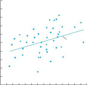
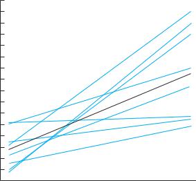
We then plot the height of the offspring against the height of their parents (Figure 5.3). In this case, we find that taller parents tend to produce taller offspring. We measure this tendency using a statistical technique called correlation (see Appendix). If offspring always exactly matched their parents, the correlation between parental height and offspring height would be 1.0. If there were no relationship, the correlation would be 0.0. In our example, the correlation is 0.41 and the slope of the line is 0.21;
|
6 |
|
|
|
|
|
|
|
|
5 |
|
|
|
|
|
|
|
(dm) |
4 |
|
|
|
|
|
|
|
height |
|
|
|
|
|
|
|
|
|
|
|
|
|
h2 |
= 0.21 |
|
|
|
|
|
|
|
|
|
|
|
Offspring |
3 |
|
|
|
|
|
|
|
|
|
|
|
|
|
|
|
|
|
2 |
|
|
|
|
|
|
|
|
1 |
1 |
2 |
3 |
4 |
5 |
6 |
7 |
|
0 |
Mean parental height (dm)
Figure 5.3 Plot of offspring height against mean height of the parents in the annual Brassica campestris (Brassicaceae) for plants grown in a greenhouse. The heritability of this trait (the slope of the line) is 0.21. (Unpublished data courtesy of Ann Evans.)
Processes of Evolution 91
there is a resemblance, but some offspring are taller than their parents, while others are shorter. Negative correlations are also possible for some traits in some species, although they are very unusual.
One measure of the heritability of a trait is the slope of the line of a regression of offspring trait values on parental values. In the above example, because we used information from both parents, the slope is exactly equal to the heritability. If we had measured only one parent, we would have information about only half of the genes being contributed to the offspring, and the slope would be one-half the heritability.
The other common way of measuring heritability is to measure the correlation among siblings. Imagine if we took two seeds from each of many plants. We could germinate the seeds and grow the pairs of siblings, measure their heights, and construct a graph much like Figure 5.3, except that now the axes would be the heights of the two siblings, and each point would represent a sibling pair. Again, the slope would measure heritability, with the exact relationship depending on whether the plants shared both parents or just one parent. We can do such an analysis with cousins or with any individuals that were related as long as we knew their relationships. Nor are we restricted to using pairs of individuals. Various statistical techniques can be used to measure heritability in groups of related plants with different degrees of relatedness.
There is a critical distinction between the heritability of a trait and whether that trait has a genetic basis. Heritability requires that phenotypic differences among individuals be due, at least in part, to genetic differences among those individuals. In Box 5A we describe a case in which height is genetically determined. In that example, some individuals have a genotype of AA, some Aa, and some aa. Instead, imagine that all individuals in the population have the same genotype, AA. Assume, however, that height also depends on the amount of nitrogen in the soil. If the population is growing in a field that varies in soil nitrogen from spot to spot, then individuals will differ in height. However, none of those phenotypic differences will be due to differences in genotypes. If we were to measure these plants, collect seeds, and raise the offspring in that same field, the correlation between parental height and offspring height would be 0, and the heritability of height in that population would be 0. Yet, there is still a gene that determines height.
This example also demonstrates that the heritability of a trait depends on the frequencies of its alleles in the population. When the frequency of A is 1.0—all individuals have the AA genotype—the heritability of the trait is 0. Thus, heritability estimates for the same trait can differ among populations, or for the same population measured at different times. Heritability estimates
92 Chapter 5
BOX 5A
PAGE PROOF: 2ND PASS
A Simple Genetic System and the Resemblance of Relatives
This example is based on the work that Gregor Mendel did in the nineteenth century with garden peas (Pisum sativa, Fabaceae), although the details have been modified for illustrative purposes. Although it is based on a simple, one-locus system, in fact nearly all traits of ecological interest are based on several to many loci. However, the same principles hold no matter how many loci affect a trait.
Consider a simple genetic system in which plant height is determined by a single diploid locus. We assume that individuals with genotype AA are tall (100 cm) and those with genotype aa are short (20 cm). We also assume that there are no environmental effects (VE = 0 and VG× E = 0) or errors of development (Ve = 0).
Case 1: Strict Additivity
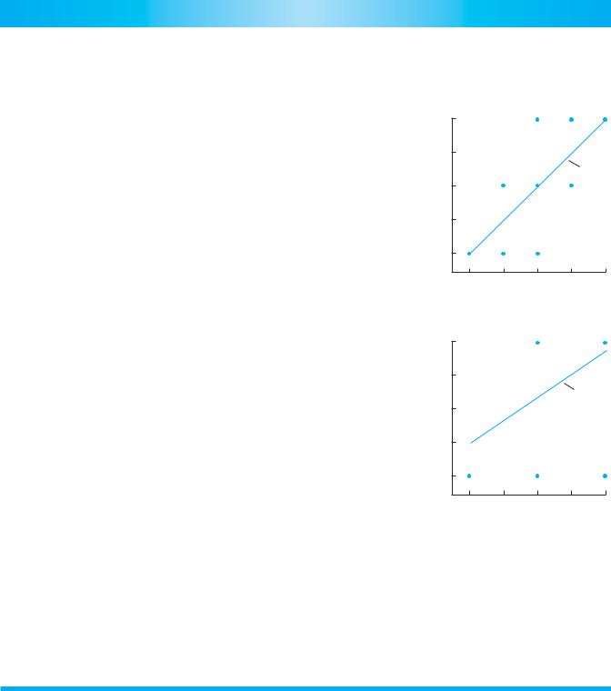
If individuals with genotype Aa have a phenotype that is exactly intermediate between AA and aa individuals, then genetic variation is strictly additive. In this case, Aa individuals would be intermediate in size (60 cm tall). Suppose we want to predict the phenotypes of the offspring of a cross. Because the effects of the alleles are strictly additive, we can do so. If both parents are tall, the cross will be AA × AA, and all offspring will be tall. If both parents are short, the cross will be aa × aa, and all offspring will be short. If one parent is tall and the other short (AA × aa), all offspring will be 60 cm tall (Aa). That is also the height that we get by averaging the parental phenotypes; the mean offspring phenotype equals the mean value of the parents’ phenotypes. If one parent is 100 cm tall and the other is 60 cm tall (AA × Aa), half the offspring will be 100 cm tall and half will be 60 cm tall. Again, the mean
value of the parents’ phenotypes, 80 cm, exactly equals the mean value of the offspring phenotype. Note that for this cross, no parent or offspring is actually at the mean height; the mean is a descriptor of the group, not a property of any particular individual. A graph of mean parental phenotype against mean offspring phenotype (part A of the accompanying figure) has a slope of 1.0. That is, the heritability of this trait is 1.0, because we can perfectly predict the average offspring phenotype from our knowledge of the parental phenotypes.
Case 2: Dominance
Now assume that A is dominant to a, such that Aa individuals are 100 cm tall. In this case, predicting offspring phenotypes becomes more difficult. If both parents are short, all offspring will be short. But if both parents are tall, their genotypes could both be Aa, or both be AA, or one AA and the other Aa. In the latter two instances, all offspring will be 100 cm tall. But if both parents are Aa, then 1/4 of the offspring will be aa and will be short. The mean offspring phenotype will be 80 cm (3/4 × 100 + 1/4 × 20), even though the mean phenotype of the parents was 100 cm. If we assume that both alleles exist with equal frequency in our population, then a graph of mean parental phenotype against mean offspring phenotype will have a slope of 0.67 (see the accompanying figure). The heritability of the trait is less than 1.0 because some of the genetic variation is nonadditive due to the dominance relationship. In other words, some offspring differ phenotypically from their parents because of the effects of dominance; if they do not inherit the dominant allele from either of their parents, they do not resemble
their parents. The exact heritability of a
(A) Strict additivity
|
100 |
|
(cm) |
h2 = 1.0 |
|
Offspring height |
60 |
|
20 |
||
|
20 |
60 |
100 |
|
Mean parental height (cm) |
|
(B) Dominance
|
100 |
(cm) |
h2 = 0.67 |
Offspring height |
60 |
|
|
|
20 |
20 |
60 |
100 |
|
Mean parental height (cm) |
|
Plot of offspring phenotype against mean parental phenotype for two genetic systems. The slope of the regression line is the heritability of the trait. (A) Strictly additive; slope = 1.
(B) Complete dominance; slope = 0.67. These heritabilities assume equal frequencies of the two alleles in the population.
trait in a population depends on both the degree of dominance and allele frequencies in the population.
are always specific to the population and environment in which they are measured.
Partitioning Phenotypic Variation
Another way of thinking about heritability is to con-
sider the various sources of phenotypic variation described above. If we measure height in a population of annual plants, it will vary due to differences in genotype, environment, and errors of development. The percentage of that variation that is caused by genetic dif-
PAGE PROOF: 2ND PASS
ferences is heritability. Mathematically, we can express this idea as follows. First, consider the total phenotypic variation, which we symbolize as VP. By a combination of experimental and statistical techniques, we can determine how much of that variation (statistical variance; see the Appendix) is due to different causes. Breaking up variation into its components is called variance partitioning. In the simplest case, we might be concerned with partitioning the phenotypic variation only into that part due to genetic variation (VG) and that part due to all other causes (Ve): VP = VG + Ve. Then, heritability would be h2 = VG/VP, the percentage of phenotypic variation that is due to genetic differences among individuals. This concept of heritability is identical to that of heritability defined as the resemblance among relatives, just a different way of measuring it.
Genetic variation can be further partitioned, however. In a diploid organism, dominance occurs when the expression of an allele depends on the properties of the other allele at that locus. In both diploid and haploid organisms, epistasis occurs when gene expression depends on the properties of alleles at other loci. The amount of genetic variation that is manifested in a population can be a result of differences in the direct expression of an allele (additive variation, VA), or to differences in combinations of alleles at each locus (dominance variation, VD), or to differences in combinations of alleles at different loci (epistatic variation, VI) (see Box 5A). Again, by various experimental and statistical procedures, we can partition this variation into its causes: VG = VA + VD + VI. If heritability is calculated as just the percentage of additive genetic variation (h2 = VA/VP), then we are speaking of narrow-sense heritability. If it is calculated as the total genetic variation (VG), then we are speaking of broad-sense heritability. This distinction is important because the response of a trait to natural selection depends on its narrow-sense heritability.
Heritability values tell us whether there is genetic variation for a trait in a population, and if so, whether there is just a little variation or a lot of variation. In terms of evolution, the amount of genetic variation may impose a constraint on evolution. If there is no genetic variation (h2 = 0), the constraint is strong. No matter how much natural selection there is on a trait, there will be no genetic response. If there is a little bit of genetic variation, the constraint is weak; there will be a genetic response, but it will be small, and evolution will proceed slowly. If there is a lot of genetic variation, there is almost no constraint.
Genotype-Environment Interactions
How does the environment influence heritability measures? Our original definition of heritability assumes that differences among individuals with different genotypes
Processes of Evolution 93
do not depend on their environment. That is, we assume that if an individual is 10% taller than another when growing in one environment, it will still be 10% taller in a different environment. But what happens when this assumption does not hold? Suppose, for example, that when a certain plant species is grown under shady conditions, all individuals are small and about the same size, but when it is grown in a sunny spot, some of those individuals are much taller than the others due to genetic differences. In other words, the genetic differences are apparent in some environments, but not in others.
These types of differences in genetic expression as a function of the environment are referred to as genotypeenvironment interactions. Genotype-environment interactions are the genetic component of phenotypic plasticity. Adding environmental effects, a full partition of the phenotypic variation of a population is
VP = VE + VG× E + VG + Ve
where VE is variation due to the environment, VG× E is variation due to genotype-environment interactions, and Ve now refers only to variation due to errors of development (Figure 5.4).
The presence of variation resulting from genotypeenvironment interactions can have large effects on heritability. Heritability is not simply a result of the genet-
|
2.0 |
|
|
1.8 |
|
|
1.6 |
|
(m) |
1.4 |
|
height |
||
1.2 |
||
Plant |
||
|
||
|
1.0 |
0.8
0.6
Low |
High |
Light environment
Figure 5.4 An example of phenotypic plasticity and geno- type-environment interaction for plants growing in high light and low light environments. In this example, cuttings were taken from individual genets and grown in each environment. Each shaded line connects the mean height for each genet in the two environments. The dashed line connects the overall means in each environment and represents VE. Variation in average heights among genets represent VG. The extent to which the shaded lines are not parallel represents VG× E.
94 Chapter 5
ic differences among individuals: those genetic differences must result in phenotypic differences. Some kinds of genetic differences among individuals never result in phenotypic differences; for example, some types of variation in noncoding regions of the DNA do not do so. In other cases, whether genetic differences result in phenotypic differences depends on the environment. When genotype-environment interaction variation is present, then the amount of expressed genetic variation may differ among environments. In the example given above, plants grown in the shade were all of similar size; in other words, phenotypic differences were minimized in that environment. If the heritability of size were measured only in the shade, we would conclude that it was very low because the amount of phenotypic variation would be low. On the other hand, if heritability were measured only in a sunny environment, it would be larger. Thus, evolution would be constrained in the shady environment because of a lack of heritable variation.
Gene-Environment Covariation
The final term that must be included in accounting for the total phenotypic variation of a trait in a population is gene-environment covariation, which is abbreviated Cov(G,E). A nonrandom relationship between any two factors is called covariation; such a relationship can be either positive or negative. Covariation is closely related to correlation; one is a mathematical transformation of the other. In this case, we are interested in covariation between genetic and environmental effects on a trait. Such covariation is often found in nature because individuals are usually not randomly distributed across environments. This is especially true of plants, as seeds often end up close to the maternal parent plant.
Positive covariation between genetic and environmental effects occurs when genetic traits are positively associated with responses to the environment. For instance, more vigorous competitors might dominate small patches of rich soil. In this case, plants that are already genetically capable of growing more rapidly will also be growing under better conditions, while slow growers will be relegated to poorer conditions. Thus, genetic differences in growth rate are exaggerated by environmental effects.
Nonrandom distribution of genotypes can act instead to minimize genetic differences. Negative covariation between genetic and environmental influences occurs when genetic and environmental influences have opposite effects. Consider a population of shrubs in which larger individuals produce more seeds. If you took the seeds of several individual shrubs and grew them all under optimal conditions in a garden, you would find a positive correlation between parental size and offspring size. In a natural population, however,
PAGE PROOF: 2ND PASS
most of the seeds will germinate in the shade of the parent plant. Because large plants produce many seeds, those seeds will be growing under crowded conditions. Plants that are genetically capable of growing larger (the offspring of the large shrubs) will be growing under poorer conditions, so genetic and environmental influences will be acting on size in opposite directions . Therefore, a negative covariation might exist.
Adding the term for covariation to the equation for phenotypic variation given above, we end up with our final equation describing phenotypic variation in a natural population:
VP = VE + VG× E + VG + Cov(G,E) + Ve
Since VP is the denominator in calculating heritability, changes in any of its components will affect the heritability of the trait.
Patterns of Adaptation
Natural selection can result in three different patterns of adaptation. First, individuals may become specialized to perform best in different environments. Within a population, for example, individuals of one phenotype might have the highest survival during periods of drought or in the driest spots, while individuals of another phenotype might survive best during wetter periods or in microhabitats with moister soil. Second, individuals might become phenotypically plastic, changing their form in different environments so as to match the most fit trait value for each set of environmental conditions. In response to changes in water availability, for example, individuals might produce leaves of different sizes and shapes. This pattern would allow them to have high survivorship during both wet and dry periods. Finally, all individuals in a population might converge on a single, intermediate phenotype that does at least passably well in all environments. This pattern is sometimes referred to as a jack-of-all-trades strategy, as in the saying “a jack-of-all-trades is a master of none.”
Which of these patterns of adaptation will prevail depends on a complex combination of factors, including how variable the environment is, how that variation is distributed in time and space, and how much genetic variation exists in the population. If the environment varies over short time periods, then phenotypic plasticity is often favored. Usually we think of phenotypic plasticity with regard to traits that become fixed during development, such as leaf shape. In aquatic plants from many unrelated families, submerged leaves are characteristically feathery and highly dissected, while emergent leaves on the same plant may have very different shapes (Figure 5.5). In water, CO2 diffusion is much slower than in air, and the highly dissected underwater leaves have increased surface areas and a smaller boundary layer (see Chapter 3), allowing