

Embedded Robotics (Thomas Braunl, 2 ed, 2006)
.pdfC. . .ONTROL. . . . . . . . . . . . . . . . . . . . . . . . . . . . . . . |
. 4 |
|
. . . . . . . . . |
losed loop control is an essential topic for embedded systems, bringing Ctogether actuators and sensors with the control algorithm in software.
The central point of this chapter is to use motor feedback via encoders for velocity control and position control of motors. We will exemplify this by a stepwise introduction of PID (Proportional, Integral, Derivative) control.
In Chapter 3, we showed how to drive a motor forward or backward and how to change its speed. However, because of the lack of feedback, the actual motor speed could not be verified. This is important, because supplying the same analog voltage (or equivalent: the same PWM signal) to a motor does not guarantee that the motor will run at the same speed under all circumstances. For example, a motor will run faster when free spinning than under load (for example driving a vehicle) with the same PWM signal. In order to control the motor speed we do need feedback from the motor shaft encoders. Feedback control is called “closed loop control” (simply called “control” in the following), as opposed to “open loop control”, which was discussed in Chapter 3.
4.1 On-Off Control
Feedback is everything
As we established before, we require feedback on a motor’s current speed in order to control it. Setting a certain PWM level alone will not help, since the motor’s speed also depends on its load.
The idea behind feedback control is very simple. We have a desired speed, specified by the user or the application program, and we have the current actual speed, measured by the shaft encoders. Measurements and actions according to the measurements can be taken very frequently, for example 100 times per second (EyeBot) or up to 20,000 times per second. The action taken depends on the controller model, several of which are introduced in the following sections. However, in principle the action always looks similar like this:
•In case desired speed is higher than actual speed:
Increase motor power by a certain degree.
•In case desired speed is lower than actual speed:
Decrease motor power by a certain degree.
5151
4 Control
In the simplest case, power to the motor is either switched on (when the speed is too low) or switched off (when the speed is too high). This control law is represented by the formula below, with:
R(t) |
|
motor output function over time t |
|
vact(t) |
|
actual measured motor speed at time t |
|
vdes(t) |
|
desired motor speed at time t |
|
KC |
|
constant control value |
|
R t |
KC |
if vact t vdes t |
|
® |
0 |
otherwise |
|
|
¯ |
||
Bang-bang
controller
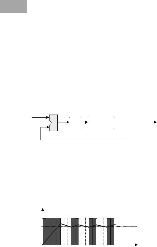
What has been defined here, is the concept of an on-off controller, also known as “piecewise constant controller” or “bang-bang controller”. The motor input is set to constant value KC if the measured velocity is too low, otherwise it is set to zero. Note that this controller only works for a positive value of vdes. The schematics diagram is shown in Figure 4.1.
desired speed
des.<act. ?
|
|
|
R(t) |
|
actual speed |
|||
|
* Kc |
|
|
|
|
Motor |
||
|
|
|
|
|
|
|
||
|
|
|
|
|
encoder |
|||
|
|
|
|
|
|
|
|
|
|
|
|
|
|
|
|
|
|
0 or 1 |
0 or Kc |
|
||||||
|
|
measurement |
||||||
|
|
|
|
|
|
|
|
|
|
feedback |
|
|
|
||||
|
|
|
|
|||||
Figure 4.1: On-off controller
The behavior over time of an on-off controller is shown in Figure 4.2. Assuming the motor is at rest in the beginning, the actual speed is less than the desired speed, so the control signal for the motor is a constant voltage. This is kept until at some stage the actual speed becomes larger than the desired speed. Now, the control signal is changed to zero. Over some time, the actual speed will come down again and once it falls below the desired speed, the control signal will again be set to the same constant voltage. This algorithm continues indefinitely and can also accommodate changes in the desired speed. Note that
vactual
R(t) |
vdesired |
t |
Figure 4.2: On-off control signal
52
On-Off Control
the motor control signal is not continuously updated, but only at fixed time intervals (e.g. every 10ms in Figure 4.2). This delay creates an overshooting or undershooting of the actual motor speed and thereby introduces hysteresis.
Hysteresis The on-off controller is the simplest possible method of control. Many technical systems use it, not limited to controlling a motor. Examples are a refrigerator, heater, thermostat, etc. Most of these technical systems use a hysteresis band, which consists of two desired values, one for switching on and one for switching off. This prevents a too high switching frequency near the desired value, in order to avoid excessive wear. The formula for an on-off controller with hysteresis is:
|
KC |
if |
vact t von t |
R t 't |
° |
if |
vact t ! voff t |
® 0 |
|||
|
¯°R t |
otherwise |
|
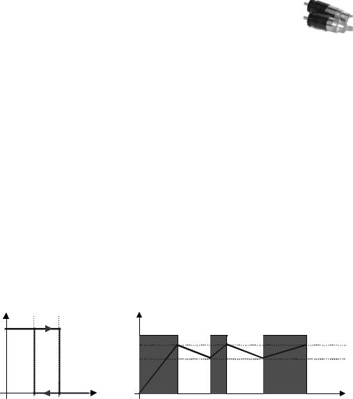
Note that this definition is not a function in the mathematical sense, because the new motor output for an actual speed between the two band limit values is equal to the previous motor value. This means it can be equal to KC or zero in this case, depending on its history. Figure 4.3 shows the hysteresis curve and the corresponding control signal.
All technical systems have some delay and therefore exhibit some inherent hysteresis, even if it is not explicitly built-in.
R(t) |
|
|
vactual |
|
|
|
R(t) |
|
|
|
voff |
|
|
|
von |
von |
voff |
vact |
t |
Figure 4.3: On-off control signal with hysteresis band
From theory to practice
Once we understand the theory, we would like to put this knowledge into practice and implement an on-off controller in software. We will proceed step by step:
1.We need a subroutine for calculating the motor signal as defined in the formula in Figure 4.1. This subroutine has to:
a.Read encoder data (input)
b.Compute new output value R(t)
c.Set motor speed (output)
2.This subroutine has to be called periodically (for example every 1/100s). Since motor control is a “low-level” task we would like this to run in the background and not interfere with any user program.
53

4 Control
Let us take a look at how to implement step 1. In the RoBIOS operating system there are functions available for reading encoder input and setting motor output (see Appendix B.5 and Figure 4.4).
1.Write a control subroutine
a.Read encoder data (INPUT)
b.Compute new output value R(t)
c.Set motor speed (OUTPUT)
See library.html:
int QUADRead(QuadHandle handle); |
|
|
Input: |
(handle) ONE decoder-handle |
|
Output: |
32bit counter-value (-2^31 .. 2^31-1) |
|
Semantics: |
Read actual Quadrature-Decoder counter, initially zero. |
|
|
Note: A wrong handle will ALSO result in a 0 counter value!! |
|
int MOTORDrive (MotorHandle handle,int speed); |
||
Input: |
(handle) logical-or of all MotorHandles which should be driven |
|
|
(speed) motor speed in percent |
|
|
Valid values: -100 - 100 (full backward to full forward) |
|
Output: |
0 |
for full stop |
(return code) 0 |
= ok |
|
Semantics: |
-1 |
= error wrong handle |
Set the given motors to the same given speed |
||
Figure 4.4: RoBIOS motor functions
The program code for this subroutine would then look like Program 4.1. Variable r_mot denotes the control parameter R(t). The dotted line has to be replaced by the control function “KC if vact<vdes” from Figure 4.1.
Program 4.1: Control subroutine framework
1void controller()
2{ int enc_new, r_mot, err;
3enc_new = QUADRead(enc1);
4...
5err = MOTORDrive(mot1, r_mot);
6if (err) printf(“error: motor”);
7}
Program 4.2 shows the completed control program, assuming this routine is called every 1/100 of a second.
So far we have not considered any potential problems with counter overflow or underflow. However, as the following examples will show, it turns out that overflow/underflow does still result in the correct difference values when using standard signed integers.
Overflow example from positive to negative values:
7F |
FF |
FF |
FC |
= |
+2147483644Dec |
80 |
00 |
00 |
06 |
= |
-6Dec |
54

On-Off Control
Program 4.2: On-off controller
Overflow and
underflow
1 |
int v_des; |
75 |
/* |
user input in ticks/s */ |
|
2 |
#define Kc |
/* |
const speed setting |
*/ |
|
3 |
|
|
|
|
|
4void onoff_controller()
5{ int enc_new, v_act, r_mot, err;
6static int enc_old;
7
8enc_new = QUADRead(enc1);
9v_act = (enc_new-enc_old) * 100;
10if (v_act < v_des) r_mot = Kc;
11 |
else r_mot = 0; |
12err = MOTORDrive(mot1, r_mot);
13if (err) printf("error: motor");
14enc_old = enc_new;
15}
The difference, second value minus first value, results in:
00 00 00 0A |
= +10Dec |
This is the correct number of encoder ticks.
Overflow Example from negative to positive values:
FF |
FF |
FF |
FD |
= |
-3Dec |
00 |
00 |
00 |
04 |
= |
+4Dec |
The difference, second value minus first value, results in +7, which is the correct number of encoder ticks.
2.Call control subroutine periodically
e.g. every 1/100 s
See library.html:
TimerHandle OSAttachTimer(int scale, TimerFnc function);
Input: |
(scale) prescale value for 100Hz Timer (1 to ...) |
Output: |
(TimerFnc) function to be called periodically |
(TimerHandle) handle to reference the IRQ-slot |
|
Semantics: |
A value of 0 indicates an error due to a full list(max. 16). |
Attach a irq-routine (void function(void)) to the irq-list. |
|
|
The scale parameter adjusts the call frequency (100/scale Hz) |
|
of this routine to allow many different applications. |
int OSDetachTimer(TimerHandle handle) |
|
Input: |
(handle) handle of a previous installed timer irq |
Output: |
0 = handle not valid |
Semantics: |
1 = function successfully removed from timer irq list |
Detach a previously installed irq-routine from the irq-list. |
|
Figure 4.5: RoBIOS timer functions
Let us take a look at how to implement step 2, using the timer functions in the RoBIOS operating system (see Appendix B.5 and Figure 4.5). There are
55
4 Control
operating system routines available to initialize a periodic timer function, to be called at certain intervals and to terminate it.
Program 4.3 shows a straightforward implementation using these routines. In the otherwise idle while-loop, any top-level user programs should be executed. In that case, the while-condition should be changed from:
while (1) /* endless loop - never returns */ to something than can actually terminate, for example:
while (KEYRead() != KEY4)
in order to check for a specific end-button to be pressed.
Program 4.3: Timer start
1int main()
2{ TimerHandle t1;
4t1 = OSAttachTimer(1, onoff_controller);
5while (1) /* endless loop - never returns */
6{ /* other tasks or idle */ }
7OSDetachTimer(t1); /* free timer, not used */
8 |
return 0; |
/* not used */ |
9 |
} |
|
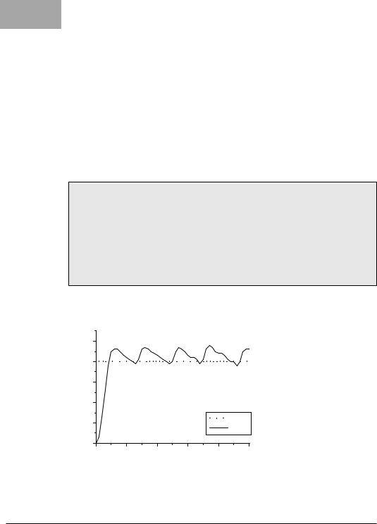
Figure 4.6 shows a typical measurement of the step response of an on-off controller. The saw-tooth shape of the velocity curve is clearly visible.
|
2500 |
|
|
|
|
|
[ticks/sec] |
2000 |
|
|
|
|
|
1500 |
|
|
|
|
|
|
|
|
|
|
|
|
|
velocity |
1000 |
|
|
|
|
|
500 |
|
|
|
|
Vdesired |
|
|
|
|
|
|
||
|
|
|
|
|
|
Vmotor |
|
0 |
|
|
|
|
|
|
0.0 |
0.1 |
0.2 |
0.3 |
0.4 |
0.5 |
time [sec]
Figure 4.6: Measured step response of on-off controller
4.2 PID Control
PID = P + I + D The simplest method of control is not always the best. A more advanced controller and almost industry standard is the PID controller. It comprises a proportional, an integral, and a derivative control part. The controller parts are introduced in the following sections individually and in combined operation.
56
PID Control
4.2.1 Proportional Controller
For many control applications, the abrupt change between a fixed motor control value and zero does not result in a smooth control behavior. We can improve this by using a linear or proportional term instead. The formula for the proportional controller (P controller) is:
R(t) = KP · (vdes(t) – vact(t))
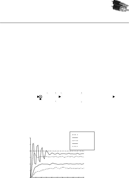
The difference between the desired and actual speed is called the “error function”. Figure 4.7 shows the schematics for the P controller, which differs only slightly from the on-off controller. Figure 4.8 shows measurements of characteristic motor speeds over time. Varying the “controller gain” KP will change the controller behavior. The higher the KP chosen, the faster the controller responds; however, a too high value will lead to an undesirable oscillating system. Therefore it is important to choose a value for KP that guarantees a fast response but does not lead the control system to overshoot too much or even oscillate.
desired speed |
|
|
|
|
actual speed |
||||
* KP |
|
|
Motor |
||||||
|
|
|
|
|
|
|
|
||
|
|
|
|
|
|
|
encoder |
||
|
|
|
|
|
|
|
|
|
|
|
|
subtract |
|
|
|
|
|||
|
|
|
|
|
|
measurement |
|||
|
|
|
|
|
|
|
|
|
|
|
|
|
|
|
|
|
|
|
|
feedback
Figure 4.7: Proportional controller
Vdesired
|
6000 |
|
|
|
|
Vmotor Kp = 0.85 |
|
|
|
|
|
|
Vmotor Kp = 0.45 |
|
|
|
|
|
|
Vmotor Kp = 0.20 |
|
|
|
|
|
|
Vmotor Kp = 0.15 |
[ticks/sec] |
4000 |
|
|
|
|
|
|
|
|
|
|
|
|
velocity |
2000 |
|
|
|
|
|
|
|
|
|
|
|
|
|
0 |
|
|
|
|
|
|
0.0 |
0.1 |
0.2 |
0.3 |
0.4 |
0.5 |
time [sec]
Figure 4.8: Step response for proportional controller
Steady state error
Note that the P controller’s equilibrium state is not at the desired velocity. If the desired speed is reached exactly, the motor output is reduced to zero, as
57
4 Control
defined in the P controller formula shown above. Therefore, each P controller will keep a certain “steady-state error” from the desired velocity, depending on the controller gain KP. As can be seen in Figure 4.8, the higher the gain KP, the lower the steady-state error. However, the system starts to oscillate if the selected gain is too high.
Program 4.4 shows the brief P controller code that can be inserted into the control frame of Program 4.1, in order to form a complete program.
Program 4.4: P controller code
1 |
e_func |
= |
v_des - v_act; |
/* |
error |
function */ |
2 |
r_mot |
= |
Kp*e_func; |
/* |
motor |
output */ |
|
|
|
|
|
|
|
4.2.2 Integral Controller
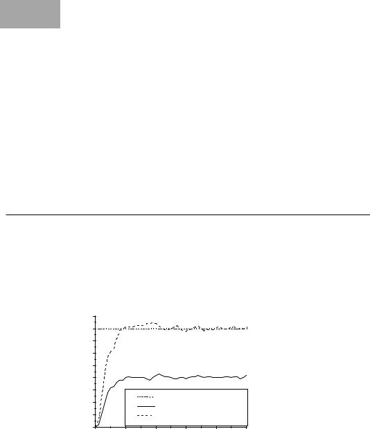
Unlike the P controller, the I controller (integral controller) is rarely used alone, but mostly in combination with the P or PD controller. The idea for the I controller is to reduce the steady-state error of the P controller. With an additional integral term, this steady-state error can be reduced to zero, as seen in the measurements in Figure 4.9. The equilibrium state is reached somewhat later than with a pure P controller, but the steady-state error has been eliminated.
|
4500 |
|
|
|
|
|
|
4000 |
|
|
|
|
|
|
3500 |
|
|
|
|
|
[ticks/sec] |
3000 |
|
|
|
|
|
2500 |
|
|
|
|
|
|
2000 |
|
|
|
|
|
|
velocity |
|
|
|
|
|
|
1500 |
|
Vdesired |
|
|
|
|
1000 |
|
|
|
|
||
|
500 |
|
P control only (Kp=0.2) |
|
||
|
|
PI control (Kp=0.2 KI=0.05) |
|
|||
|
|
|
|
|||
|
0 |
|
|
|
|
|
|
0.0 |
0.1 |
0.2 |
0.3 |
0.4 |
0.5 |
time [sec]
Figure 4.9: Step response for integral controller
When using e(t) as the error function, the formula for the PI controller is: R(t) = KP · [ e(t) + 1/TI · 0³t e(t)dt ]
We rewrite this formula by substituting QI = KP/TI, so we receive independent additive terms for P and I:
R(t) = KP · e(t) + QI · 0³t e(t)dt
58

PID Control
Naive approach
Proper PI implementation
The naive way of implementing the I controller part is to transform the integration into a sum of a fixed number (for example 10) of previous error values. These 10 values would then have to be stored in an array and added for every iteration.
The proper way of implementing a PI controller starts with discretization, replacing the integral with a sum, using the trapezoidal rule:
R |
= K |
|
· e |
+ |
Q |
· t |
· |
n |
ei ei 1 |
P |
¦ |
------------------- |
|||||||
|
n |
|
n |
I |
delta |
|
2 |
||
|
|
|
|
|
|
|
|
i 1 |
|
Now we can get rid of the sum by using Rn–1, the output value preceding Rn:
Limit controller output values!
Rn – Rn–1 = KP · (en – en–1) + QI · tdelta · (en + en–1)/2 Therefore (substituting KI for QI · tdelta):
Rn = Rn–1 + KP · (en – en–1) + KI · (en + en–1)/2
So we only need to store the previous control value and the previous error value to calculate the PI output in a much simpler formula. Here it is important to limit the controller output to the correct value range (for example -100 .. +100 in RoBIOS) and also store the limited value for the subsequent iteration. Otherwise, if a desired speed value cannot be reached, both controller output and error values can become arbitrarily large and invalidate the whole control process [Kasper 2001].
Program 4.5 shows the program fragment for the PI controller, to be inserted into the framework of Program 4.1.
Program 4.5: PI controller code
1 |
static |
int r_old=0, e_old=0; |
||
2 ... |
= v_des - |
v_act; |
|
|
3 |
e_func |
|
||
4 |
r_mot |
= r_old + |
Kp*(e_func-e_old) + Ki*(e_func+e_old)/2; |
|
5 |
r_mot = min(r_mot, +100); |
/* limit output */ |
||
6 |
r_mot = max(r_mot, -100); |
/* limit output */ |
||
7 |
r_old |
= r_mot; |
|
|
8 |
e_old |
= e_func; |
|
|
|
|
|
|
|
4.2.3 Derivative Controller
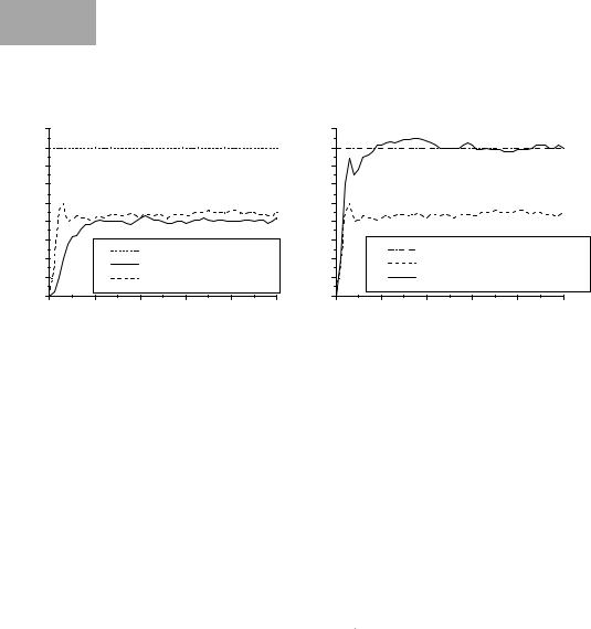
Similar to the I controller, the D controller (derivative controller) is rarely used by itself, but mostly in combination with the P or PI controller. The idea for adding a derivative term is to speed up the P controller’s response to a change of input. Figure 4.10 shows the measured differences of a step response between the P and PD controller (left), and the PD and PID controller (right). The PD controller reaches equilibrium faster than the P controller, but still has
59
4 Control
a steady-state error. The full PID controller combines the advantages of PI and PD. It has a fast response and suffers no steady-state error.
|
4500 |
|
|
|
|
|
4500 |
|
4000 |
|
|
|
|
|
4000 |
|
3500 |
|
|
|
|
|
3500 |
[ticks/sec] |
3000 |
|
|
|
|
[ticks/sec] |
3000 |
2500 |
|
|
|
|
2500 |
||
2000 |
|
|
|
|
2000 |
||
velocity |
1500 |
|
Vdesired |
|
|
velocity |
1500 |
1000 |
|
|
|
1000 |
|||
|
|
P control only (Kp |
=0.2) |
|
|||
|
500 |
|
|
500 |
|||
|
|
PD control (KP=0.2 KD=0.3) |
|
||||
|
|
|
|
|
|||
|
0 |
|
|
|
|
|
0 |
|
0.0 |
0.1 |
0.2 |
0.3 |
0.4 |
0.5 |
|
|
|
Vdesired |
|
|
|
|
|
PD control (Kp=0.2 KD=0.3) |
|
||
|
|
PID control (Kp=0.2 KI=0.05 KD=0.3) |
|||
0.0 |
0.1 |
0.2 |
0.3 |
0.4 |
0.5 |
time [sec] |
time [sec] |
Figure 4.10: Step response for derivative controller and PID controller
When using e(t) as the error function, the formula for a combined PD controller is:
R(t) = KP · [ e(t) + TD · de(t)/dt]
The formula for the full PID controller is:
R(t) = KP · [ e(t) + 1/TI · 0³t e(t)dt + TD · de(t)/dt ]
Again, we rewrite this by substituting TD and TI, so we receive independent additive terms for P, I, and D. This is important, in order to experimentally adjust the relative gains of the three terms.
R(t) = KP · e(t) + QI · 0³t e(t)dt + QD · de(t)/dt
Using the same discretization as for the PI controller, we will get:
R |
= K |
|
· e |
|
+ |
Q |
· t |
|
· |
n |
ei ei 1 |
+ Q |
/ t |
· (e – e |
|
) |
P |
n |
delta |
¦ |
------------------- |
n–1 |
|||||||||||
|
n |
|
|
I |
|
|
2 |
D |
delta |
n |
|
|||||
|
|
|
|
|
|
|
|
|
|
i 1 |
|
|
|
|
|
|
Again, using the difference between subsequent controller outputs, this results in:
Rn – Rn–1 = KP · (en – en–1) + QI · tdelta · (en + en–1)/2
+ QD / tdelta · (en – 2·en–1 + en–2) Finally (substituting KI for QI · tdelta and KD for QD / tdelta):
Complete Rn = Rn–1 + KP · (en – en–1) + KI · (en + en–1)/2 + KD · (en - 2·en–1 + en–2)
PID formula
Program 4.6 shows the program fragment for the PD controller, while Program 4.7 shows the full PID controller. Both are to be inserted into the framework of Program 4.1.
60