Embedded Robotics (Thomas Braunl, 2 ed, 2006)

22 Behavior-Based Systems

22.8 Experiments

The task set for the evolution of our behavior-based system was to make a robot detect a ball and drive toward it. The driving environment is a square area with the ball in the middle and the robot placed at a random position and orientation. This setup is similar to the one used in Section 21.5.

The evolution has been run with minimal settings, namely 20 generations with 20 individuals. In order to guarantee a fair evaluation, each individual is run three times with three different original distances from the ball. The same three distance values are used for the whole population, while the individual robot placement is still random, i.e. along a circle around the ball.

Program 22.5: Fitness function for ball tracking

1fitness = initDist - b_distance();

2if (fitness < 0.0) fitness = 0.0;

The fitness function used is shown in Program 22.5. We chose only the improvement in distance toward the ball for the fitness function, while negative values are reset to zero. Note that only the desired outcome of the robot getting close to the ball has been encoded and not the robot’s performance during the driving. For example, it would also have been possible to increase an individual’s fitness whenever the ball is in its field of view – however, we did not want to favor this selection through hard-coding. The robot should discover this itself through evolution. Experiments also showed that even a simpler neural network with 2u4u3 nodes is sufficient for evolving this task, instead of 2u6u3.

Figure 22.9: Robot driving result

340

Experiments

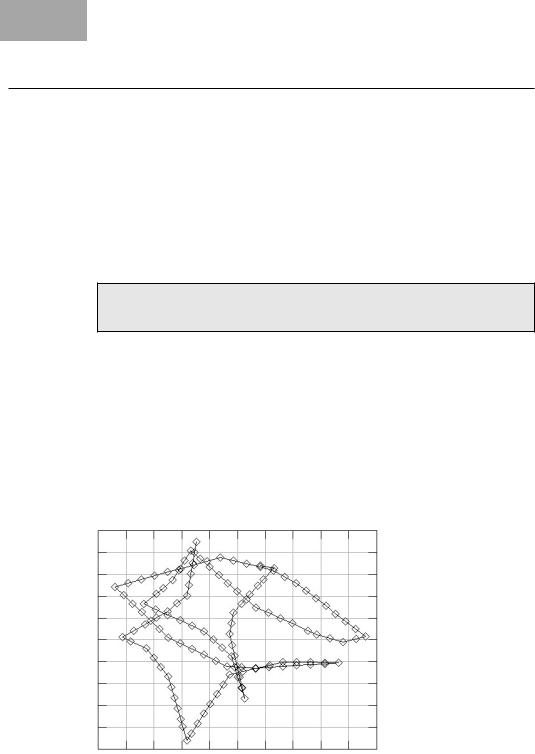
This elementary fitness function worked surprisingly well. The robots learned to detect the ball and drive toward it. However, since there are no incentives to stop once the ball has been approached, most high-scoring robots continued pushing and chasing the ball around the driving environment until the maximum simulation time ran out. Figure 22.9 shows typical driving results obtained from the best performing individual after 11 generations. The robot is able to find the ball by rotating from its starting position until it is in its field of view, and can then reliably track the ball while driving toward it, and will continue to chase the ball that is bouncing off the robot and off the walls.

Figure 22.10: Fitness development over generations

Figure 22.11: Individual runs of best evolved behavioral controller

341

22 Behavior-Based Systems

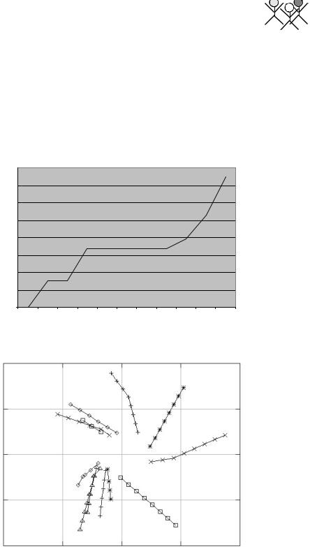
Figure 22.10 shows the development of the maximum fitness over 10 generations. The maximum fitness increases consistently and finally reaches a level of acceptable performance.

This experiment can be extended if we want to make the robot stop in front of the ball, or change to a different behavioral pattern (for example goal kicking). What needs to be done is to change the fitness function, for example by adding a bonus for stopping in a time shorter than the maximum allowed simulation time, and to extend the neural network with additional output (and hidden) nodes. Care needs to be taken that only robots with a certain fitness for approaching the ball get the time bonus, otherwise “lazy” robots that do not move and stop immediately would be rewarded. Figure 22.11 shows several runs of the best evolved behavioral controller. This state was reached after 20 generations; the simulation is halted once the robot gets close to the ball.

22.9 References

AGRE, P., CHAPMAN, D. What are plans for?, Robotics and Autonomous Systems, vol. 6, no. 1-2, 1990, pp. 17-34 (18)

ARKIN, R. Behavior Based Robotics, MIT Press, Cambridge MA, 1998

ARKIN, R., BALCH, T. AuRA: Principles and Practice in Review, Journal of Experimental and Theoretical Artificial Intelligence, vol. 9, no. 2-3, 1997, pp. 175-189 (15)

BALCH, T., ARKIN, R., Communication in Reactive Multiagent Robotic Systems, Autonomous Robots, vol. 1, no. 1, 1994, pp. 27-52 (26)

BALCH T. TeamBots simulation environment, available from http://www. teambots.org, 2006

BRAITENBERG, V. Vehicles, experiments in synthetic psychology, MIT Press, Cambridge MA, 1984

BROOKS, R. A Robust Layered Control System For A Mobile Robot, IEEE Journal of Robotics and Automation, vol. 2, no.1, 1986, pp. 14-23 (7)

DU J., BRÄUNL, T. Collaborative Cube Clustering with Local Image Processing, Proc. of the 2nd Intl. Symposium on Autonomous Minirobots for Research and Edutainment, AMiRE 2003, Brisbane, Feb. 2003, pp. 247-248 (2)

GURNEY, K. Neural Nets, UCL Press, London, 2002

ISKE, B., RUECKERT, U. Cooperative Cube Clustering using Local Communication, Autonomous Robots for Research and Edutainment - AMiRE 2001, Proceedings of the 5th International Heinz Nixdorf Symposium, Paderborn, Germany, 2001, pp. 333-334 (2)

MORAVEC, H. Mind Children: The Future of Robot and Human Intelligence, Harvard University Press, Cambridge MA, 1988

342

References

STEELS, L., BROOKS, R. Building Agents out of Autonomous Behavior Systems, in L. Steels, R. Brooks (Eds.), The Artificial Life Route to AI: Building Embodied, Situated Agents, Erlbaum Associates, Hillsdale NJ, 1995

VENKITACHALAM, D. Implementation of a Behavior-Based System for the Control of Mobile Robots, B.E. Honours Thesis, The Univ. of Western Australia, Electrical and Computer Eng., supervised by T. Bräunl, 2002

WAGGERSHAUSER, A. Simulating small mobile robots, Project Thesis, Univ. Kaiserslautern / The Univ. of Western Australia, supervised by T. Bräunl and E. von Puttkamer, 2002

343

Designing or optimizing control systems for legged locomotion is a complex and time consuming process. Human engineers can only produce and evaluate a limited number of configurations, although

there may be numerous competing designs that should be investigated. Automation of the controller design process allows the evaluation of thousands of competing designs, without requiring prior knowledge of the robot’s walking mechanisms [Ledger 1999]. Development of an automated approach requires the implementation of a control system, a test platform, and an adaptive method for automated design of the controller. Thus, the implemented control system must be capable of expressing control signals that can sufficiently describe the desired walking pattern. Furthermore, the selected control system should be simple to integrate with the adaptive method.

One possible method for automated controller design is to utilize a spline controller and evolve its control parameters with a genetic algorithm [Boeing, Bräunl 2002], [Boeing, Bräunl 2003]. To decrease the evolution time and remove the risk of damaging robot hardware during the evolution, a dynamic mechanical simulation system can be employed.

23.1 Splines

Splines are a set of special parametric curves with certain desirable properties. They are piecewise polynomial functions, expressed by a set of control points. There are many different forms of splines, each with their own attributes [Bartels, Beatty, Barsky 1987]; however, there are two desirable properties:

•Continuity, so the generated curve smoothly connects its parts.

•Locality of the control points, so the influence of a control point is limited to a neighborhood region.

345345

23 Evolution of Walking Gaits

The Hermite spline is a special spline with the unique property that the curve generated from the spline passes through the control points that define the spline. Thus, a set of pre-determined points can be smoothly interpolated by simply setting these points as control points for the Hermite spline. Each segment of the curve is dependent on only a limited number of the neighboring control points. Thus, a change in the position of a distant control point will not alter the shape of the entire spline. The Hermite spline can also be constrained so as to achieve CK–2 continuity.

The function used to interpolate the control points, given starting point p1, ending point p2, tangent values t1 and t2, and interpolation parameter s, is shown below:

f(s) = h1p1 + h2p2 + h3t1 + h4t2 where

h1 = 2s3 – 3s2 + 1

h2 = –2s3 + 3s2 h3 = s3 – 2s2 + s h4 = s3 – s2

for 0 d s d 1

Program 23.1 shows the routine utilized for evaluating splines. Figure 23.1 illustrates the output from this function when evaluated with a starting point at one, with a tangent of zero, and an ending point of zero with a tangent of zero. The Hermite_Spline function was then executed with s ranging from zero to one.

Program 23.1: Evaluating a simple cubic Hermite spline section

1float Hermite_Spline(float s) {

2float ss=s*s;

3float sss=s*ss;

12return value;

13}

23.2Control Algorithm

346

Control Algorithm

Hermite(s)

s

Figure 23.1: Cubic Hermite spline curve

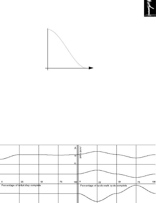
spline controller consists of a set of joined Hermite splines. The first set contains robot initialization information, to move the joints into the correct positions and enable a smooth transition from the robot’s starting state to a traveling state. The second set of splines contains the cyclic information for the robot’s gait. Each spline can be defined by a variable number of control points, with variable degrees of freedom. Each pair of a start spline and a cyclic spline corresponds to the set of control signals required to drive one of the robot’s actuators.

An example of a simple spline controller for a robot with three joints (three degrees of freedom) is illustrated in Figure 23.2. Each spline indicates the controller’s output value for one actuator.

Figure 23.2: Spline joint controller

There are a number of advantages offered by Hermite spline controllers. Since the curve passes through all control points, individual curve positions can be pre-determined by a designer. This is especially useful in situations where the control signal directly corresponds to angular, or servo, positions. Program 23.2 provides a simplified code snippet for calculating the position values for a one-dimensional spline.

347

23 Evolution of Walking Gaits

Program 23.2: Evaluating a concatenated Hermite spline

6float secpos;

7secpos=s*(nsec-1);

8sect=(int)floorf(secpos);

9z=fmodf(secpos,1);

10return hs[sect].Eval(z);

11}

There is a large collection of evidence that supports the proposition that most gaits for both animals and legged robots feature synchronized movement [Reeve 1999]. That is, when one joint alters its direction or speed, this change is likely to be reflected in another limb. Enforcing this form of constraint is far simpler with Hermite splines than with other control methods. In order to force synchronous movement with a Hermite spline, all actuator control points must lie at the same point in cycle time. This is because the control points represent the critical points of the control signal when given default tangent values.

23.3 Incorporating Feedback

Most control methods require a form of feedback in order to correctly operate (see Chapter 10). Spline controllers can achieve walking patterns without the use of feedback; however, incorporating sensory information into the control system allows a more robust gait. The addition of sensory information to the spline control system enabled a bipedal robot to maneuver on uneven terrain.

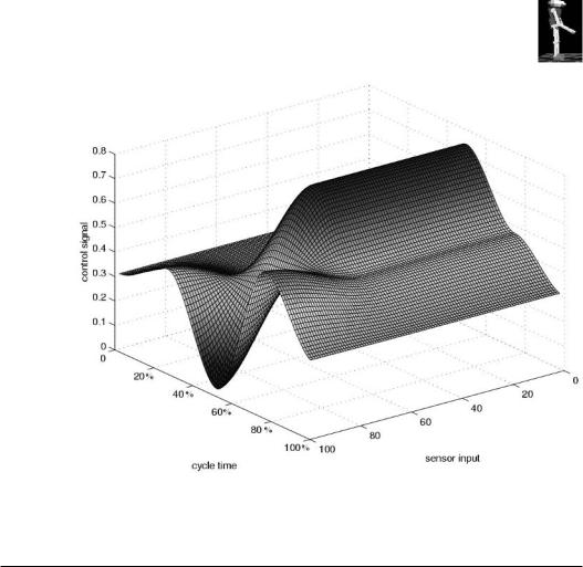
In order to incorporate sensor feedback information into the spline controller, the controller is extended into another dimension. The extended control points specify their locations within both the gait’s cycle time and the feedback value. This results in a set of control surfaces for each actuator. Extending the controller in this form significantly increases the number of control points required. Figure 23.3 illustrates a resulting control surface for one actuator.

The actuator evaluates the desired output value from the enhanced controller as a function of both the cycle time and the input reading from the sensor. The most appropriate sensory feedback was found to be an angle reading from an inclinometer (compare Section 2.8.3) placed on the robot’s central body (torso). Thus, the resultant controller is expressed in terms of the percentage cycle time, the inclinometer’s angle reading, and the output control signal.

348

Controller Evolution

Figure 23.3: Generic extended spline controller

23.4 Controller Evolution

Genetic algorithms can be applied to automate the design of the control system. To achieve this, the parameters for the control system need to be encoded in a format that can be evolved by the genetic algorithm. The parameters for the spline control system are simply the position and tangent values of the control points that are used to describe the spline. Thus, each control point has three different values that can be encoded:

•Its position in the cycle time (i.e. position along the x-axis)

•The value of the control signal at that time (i.e. position along the y-axis)

•The tangent value

To allow these parameters to evolve with a genetic algorithm in minimal time, a more compact format of representing the parameters is desired. This can be achieved by employing fixed point values.

For example, if we wanted to encode the range [0..1] using 8bit fixed point values, then the 8 bits can represent any integer value from 0 to 255. By simply

349

23 Evolution of Walking Gaits

dividing this value by 255, we can represent any number ranging from 0 to 1, with an accuracy of 0.004 (1/256).

The curve shown in Figure 23.1 was generated by a one-dimensional spline function, with the first control point (s = 0) at position 1 with tangent value of 0, and the second control point (s = 1) at position 0 with tangent value of 0. If an encoding which represented each value as an 8bit fixed point number from 0 to 1 is used, then the control parameters in this case would be represented as a string of 3 bytes with values of [0, 255, 0] for the first control point’s position and tangent, and [255, 0, 0] for the second control point’s position and tangent.

Thus, the entire spline controller can be directly encoded using a list of control point values for each actuator. An example structure to represent this information is shown in Program 23.3.

Program 23.3: Full direct encoding structures

1struct encoded_controlpoint {

2unsigned char x,y,tangent;

3};

4

5struct encoded_splinecontroller {

6encoded_controlpoint

7initialization_spline[num_splines][num_controlpoints];

8encoded_controlpoint

Staged evolution There are a number of methods for optimizing the performance of the genetic algorithm. One method for increasing the algorithm’s performance is staged evolution. This concept is an extension to “Behavioural Memory”, and was first applied to controller evolution by [Lewis, Fagg, Bekey 1994]. Staged evolution divides a problem task into a set of smaller, manageable challenges that can be sequentially solved. This allows an early, approximate solution to the problem to be solved. Then, incrementally increasing the complexity of the problem provides a larger solution space for the problem task and allows for further refinements of the solution. Finally, after solving all the problem’s subtasks, a complete solution can be determined. Solving the sequence of subtasks is typically achieved in less time than required if the entire problem task is tackled without decomposition.

This optimization technique can also be applied to the design of the spline controller. The evolution of the controller’s parameters can be divided into the following three phases:

1.Assume that each control point is equally spaced in the cycle time. Assume the tangent values for the control points are at a default value. Only evolve the parameters for the control points’ output signal (y-axis).

2.Remove the restriction of equidistant control points, and allow the control points to be located at any point within the gait time (x-axis).

350