Embedded Robotics (Thomas Braunl, 2 ed, 2006)

Example Evolution

The initial population, encodings, and fitnesses are given in Table 20.1. Note that chromosomes x = 2 and x = 10 have equal fitness values, hence their relative ranking is an arbitrary choice.

The genetic algorithm we use has a simple form of selection and reproduction. The top performing chromosome is reproduced and preserved for use in the next iteration of the algorithm. It replaces the lowest performing chromosome, which is removed from the population altogether. Hence we remove x = 31 from selection.

The next step is to perform crossover between the chromosomes. We randomly pair the top four ranked chromosomes and determine whether they are subject to crossover by a non-deterministic probability. In this example, we have chosen a crossover probability of 0.5, easily modeled by a coin toss. The random pairings selected are ranked chromosomes (1,4) and (2,3). Each pair of chromosomes will undergo a single random point crossover to produce two new chromosomes.

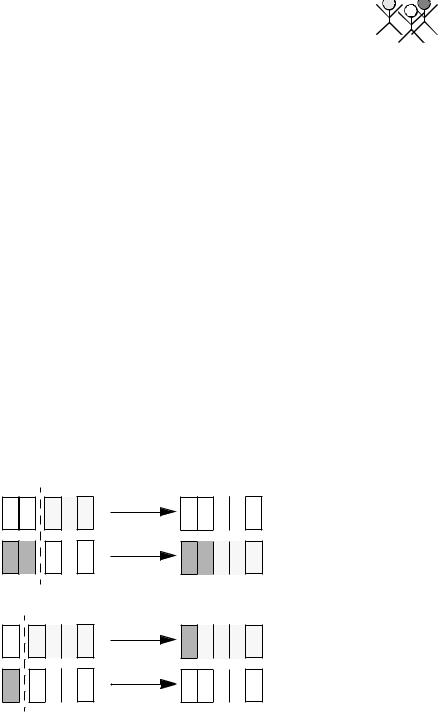
As described earlier, the single random point crossover operation selects a random point to perform the crossover. In this iteration, both pairs undergo crossover (Figure 20.8).

The resulting chromosomes from the crossover operation are as follows:

(1)00|010 po 00100 = 4

(4)10|100 no 10010 = 18

(2)0|1010 po 00000 = 0

(3)0|0000 no 01010 = 10

Crossover point

Crossover point

Figure 20.8: Crossover

Note that in the case of the second crossover, because the first bit is identical in both strings the resulting chromosomes are the same as the parents. This is effectively equivalent to no crossover operation occurring. After one itera-

299

20 Genetic Algorithms

tion we can see the population has converged somewhat toward the optimal answer. We now repeat the evaluation process with our new population (Table 20.2).

(x = 18). Our random pairings this time are ranked chromosomes (1, 2) and (3, 4). This time, only pair (3, 4) has been selected by a random process to cross over, and (1, 2) is selected for mutation. It is worth noting that the (1, 2) pair had the potential to produce the optimal solution x = 6 if it had undergone crossover. This missed opportunity is characteristic of the genetic algorithm’s non-deterministic nature: the time taken to obtain an optimal solution cannot be accurately foretold. The mutation of (2), however, reintroduced some of the lost bit-string representation. With no mutate operator the algorithm would no longer be capable of representing odd values (bit strings ending with a one).

Mutation of (1) and (2)

(1)00100 o 00000 = 0

(2)00010 o 00011 = 3

Crossover of pair (3, 4)

(3)01|010 po 01000 = 8

(4)00|000 no 00010 = 2

The results of the next population fitness evaluation are presented in Table 20.3.

As before, chromosome x = 0 is removed and x = 4 is retained. The selected pairs for crossover are (1, 3) and (1, 4), of which only (1, 4) actually undergoes crossover:

(1) 001|00 po 00110 = 6

(4) 000|10 no 00000 = 0

The optimal solution of x = 6 has been obtained. At this point, we can stop the genetic algorithm because we know this is the optimal solution. However, if we let the algorithm continue, it should eventually completely converge to

300

20 Genetic Algorithms

Program 20.1: Gene header

tions that all parameter types must implement so that they can be generically manipulated consistently externally. An excerpt of the Gene header file is given in Program 20.1.

Program 20.2: Chromosome header

1class Chromosome

2{

3// Return the number of genes in this chromosome.

4int getNumGenes();

5// Set the gene at a specified index.

6int setGene(int index, Gene* gene);

7// Add a gene to the chromosome.

8int addGene(Gene* gene);

9// Get a gene at a specified index.

10Gene* getGene(int index);

11// Set fitness of chromosome as by ext. fitness function

12void setFitness(double value);

13// Retrieve the fitness of this chromosome

14double getFitness(void);

15// Perform single crossover with a partner chromosome

16virtual void crossover(Chromosome* partner);

17// Perform a mutation of the chromosome

18virtual void mutate(void);

19// Return a new identical copy of this chromosome

20Chromosome& clone(void);

21};

302

Implementation of Genetic Algorithms

The chromosome class stores a collection of genes in a container class. It provides access to basic crossover and mutation operators. These can be overridden and extended with more complex operators as described earlier. An excerpt of the chromosome header file is given in Program 20.2.

Finally, the population class (Program 20.3) is the collection of Chromosomes comprising a full population. It performs the iterative steps of the genetic algorithm, evolving its own population of Chromosomes by invoking their defined operators. Access to individual Chromosomes is provided, allowing evaluation of terminating conditions through an external routine.

Program 20.3: Population class

1class Population

2{// Initialise population with estimated no. chromosomes

10

11// Set population parameters

12void setCrossover(float rate);

13void setMutation(float rate);

14void setDecease(float rate);

16// Create new pop. with selection, crossover, mutation

17virtual void evolveNewPopulation(void);

18int getPopulationSize(void);

19Chromosome& getChromosome(int index);

21// Print pop. state, (chromosome vals & fitness stats)

22void printState(void);

24// Sort population according to fitness,

25void sortPopulation(void);

26};

As an example of using these classes, Program 20.4 shows an excerpt of code to solve our quadratic problem, using a derived integer representation class GeneInt and the Chromosome and Population classes described above.

303

20 Genetic Algorithms

Program 20.4: Main program

1int main(int argc, char *argv[])

2{ int i;

3

4GeneInt genes[5];

5Chromosome* chromosomes[5];

6Population population;

7

8population.setCrossover(0.5f);

9population.setDecease(0.2f);

10population.setMutation(0.0f);

12// Initialise genes and add them to our chromosomes,

13// then add the chromosomes to the population

14for(i=0; i<5; i++) {

15genes[i].setData((void*) rand()%32);

16chromosomes[i].addGene(&genes[i]);

17population.addChromosome(&chromosomes[i]);

18}

19

20// Continually run the genetic algorithm until the

21// optimal solution is found by the top chromosome

23i = 0;

24do {

25printf("Iteration %d", i++);

26population.evolveNewPopulation();

27population.printState();

28} while((population.getChromosome(0)).getFitness()!=0);

30// Finished

31return 0;

32}

20.6References

BEASLEY, D., BULL, D., MARTIN, R. An Overview of Genetic Algorithms: Part 1, Fundamentals, University Computing, vol. 15, no. 2, 1993a, pp. 58-69 (12)

BEASLEY, D., BULL, D., MARTIN, R. An Overview of Genetic Algorithms: Part 2, Research Topics, University Computing, vol. 15, no. 4, 1993b, pp. 170-181 (12)

BEAULIEU, J., GAGNÉ, C. Open BEAGLE – A Versatile Evolutionary Computation Framework, Département de génie électrique et de génie informatique, Université Laval, Québec, Canada, http://www.gel.ulaval.

ca/~beagle/, 2006

304

References

DARWIN, C. On the Origin of Species by Means of Natural Selection, or Preservation of Favoured Races in the Struggle for Life, John Murray, London, 1859

GALIB Galib – A C++ Library of Genetic Algorithm Components, http:// lancet.mit.edu/ga/, 2006

GOLDBERG, D. Genetic Algorithms in Search, Optimization and Machine Learning, Addison-Wesley, Reading MA, 1989

HARVEY, I., HUSBANDS, P., CLIFF, D. Issues in Evolutionary Robotics, in J. Meyer, S. Wilson (Eds.), From Animals to Animats 2, Proceedings of the Second International Conference on Simulation of Adaptive Behavior, MIT Press, Cambridge MA, 1993

IJSPEERT, A. Evolution of neural controllers for salamander-like locomotion, Proceedings of Sensor Fusion and Decentralised Control in Robotics Systems II, 1999, pp. 168-179 (12)

LANGTON, C. (Ed.) Artificial Life – An Overview, MIT Press, Cambridge MA, 1995

LEWIS, M., FAGG, A., BEKEY, G. Genetic Algorithms for Gait Synthesis in a Hexapod Robot, in Recent Trends in Mobile Robots, World Scientific, New Jersey, 1994, pp. 317-331 (15)

RAM, A., ARKIN, R., BOONE, G., PEARCE, M. Using Genetic Algorithms to Learn Reactive Control Parameters for Autonomous Robotic Navigation, Journal of Adaptive Behaviour, vol. 2, no. 3, 1994, pp. 277-305 (29)

VENKITACHALAM, D. Implementation of a Behavior-Based System for the Control of Mobile Robots, B.E. Honours Thesis, The Univ. of Western Australia, Electrical and Computer Eng., supervised by T. Bräunl, 2002

305

enetic programming extends the idea of genetic algorithms discussed Gin Chapter 20, using the same idea of evolution going back to Darwin [Darwin 1859]. Here, the genotype is a piece of software, a directly executable program. Genetic programming searches the space of possible computer programs that solve a given problem. The performance of each individual program within the population is evaluated, then programs are selected according to their fitness and undergo operations that produce a new set of programs. These programs can be encoded in a number of different programming languages, but in most cases a variation of Lisp [McCarthy et al. 1962] is cho-

sen, since it facilitates the application of genetic operators.

The concept of genetic programming was introduced by Koza [Koza 1992]. For further background reading see [Blickle, Thiele 1995], [Fernandez 2006], [Hancock 1994], [Langdon, Poli 2002].

21.1 Concepts and Applications

The main concept of genetic programming is its ability to create working programs without the full knowledge of the problem or the solution. No additional encoding is required as in genetic algorithms, since the executable program itself is the phenotype. Other than that, genetic programming is very similar to genetic algorithms. Each program is evaluated by running it and then assigning a fitness value. Fitness values are the base for selection and genetic manipulation of a new generation. As for genetic algorithms, it is important to maintain a wide variety of individuals (here: programs), in order to fully cover the search area.

Koza summarizes the steps in genetic programming as follows [Koza 1992]:

307307

21 Genetic Programming

308

Lisp

Table 21.1: Initial population sizes

21.2 Lisp

S-Expression Lists may be nested and are not only the representation for data structures, but also for program code as well. Lists that start with an operator, such as (+ 1 2), are called S-expressions. An S-expression can be evaluated by the Lisp interpreter (Figure 21.1) and will be replaced by a result value (an atom or a list, depending on the operation). That way, a program execution in a procedural programming language like C will be replaced by a function call in Lisp:

309