Embedded Robotics (Thomas Braunl, 2 ed, 2006)

Simulated versus Real Maze Program

Figure 15.9: Shortest path for position [y,x] = [1,2]

Figure 15.10: Simulated maze solving

changes to improve the application’s robustness and fault tolerance, before we eventually try it on a real robot in a maze environment.

What needs to be added to the previously shown maze program can be described by the term fault tolerance. We must not assume that a robot has turned 90° degrees after we give it the corresponding command. It may in fact

227

15 Maze Exploration

have turned only 89° or 92°. The same holds for driving a certain distance or for sensor readings. The logic of the program does not need to be changed, only the driving routines.

The best way of making our maze program fault tolerant is to have the robot continuously monitor its environment while driving (Figure 15.10). Instead of issuing a command to drive straight for a certain distance and wait until it is finished, the robot should constantly measure the distance to the left and right wall while driving and continuously correct its steering while driving forward. This will correct driving errors as well as possible turning errors from a previous change of direction. If there is no wall to the left or the right or both, this information can be used to adjust the robot’s position inside the square, i.e. avoiding driving too far or too short (Figure 15.11). For the same reason, the robot needs to constantly monitor its distance to the front, in case there is a wall.

Figure 15.11: Adaptive driving using three sensors

15.4 References

ALLAN, R. The amazing micromice: see how they won, IEEE Spectrum, Sept. 1979, vol. 16, no. 9, pp. 62-65 (4)

BILLINGSLEY, J. Micromouse - Mighty mice battle in Europe, Practical Computing, Dec. 1982, pp. 130-131 (2)

BRÄUNL, T. Research Relevance of Mobile Robot Competitions, IEEE Robotics and Automation Magazine, vol. 6, no. 4, Dec. 1999, pp. 32-37 (6)

CHRISTIANSEN, C. Announcing the amazing micromouse maze contest, IEEE Spectrum, vol. 14, no. 5, May 1977, p. 27 (1)

HINKEL, R. Low-Level Vision in an Autonomous Mobile Robot, EUROMICRO 1987; 13th Symposium on Microprocessing and Microprogramming, Portsmouth England, Sept. 1987, pp. 135-139 (5)

KOESTLER, A., BRÄUNL, T., Mobile Robot Simulation with Realistic Error Models, International Conference on Autonomous Robots and Agents, ICARA 2004, Dec. 2004, Palmerston North, New Zealand, pp. 46-51

(6)

228

Mapping an unknown environment is a more difficult task than the maze exploration shown in the previous chapter. This is because, in a maze, we know for sure that all wall segments have a certain

length and that all angles are at 90°. In the general case, however, this is not the case. So a robot having the task to explore and map an arbitrary unknown environment has to use more sophisticated techniques and requires higher-pre- cision sensors and actuators as for a maze.

16.1 Mapping Algorithm

Several map generation systems have been presented in the past [Chatila 1987], [Kampmann 1990], [Leonard, Durrant-White 1992], [Melin 1990], [Piaggio, Zaccaria 1997], [Serradilla, Kumpel 1990]. While some algorithms are limited to specific sensors, for example sonar sensors [Bräunl, Stolz 1997], many are of a more theoretical nature and cannot be directly applied to mobile robot control. We developed a practical map generation algorithm as a combination of configuration space and occupancy grid approaches. This algorithm is for a 2D environment with static obstacles. We assume no prior information about obstacle shape, size, or position. A version of the “DistBug” algorithm [Kamon, Rivlin 1997] is used to determine routes around obstacles. The algorithm can deal with imperfect distance sensors and localization errors [Bräunl, Tay 2001].

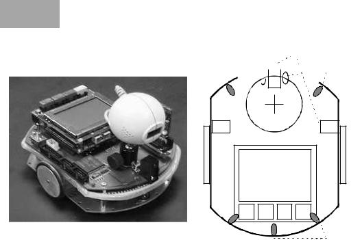
For implementation, we are using the robot Eve, which is the first EyeBotbased mobile robot. It uses two different kinds of infrared sensors: one is a binary sensor (IR-proxy) which is activated if the distance to an obstacle is below a certain threshold, the other is a position sensitive device (IR-PSD) which returns a distance value to the nearest obstacle. In principle, sensors can be freely positioned and oriented around the robot. This allows testing and comparison of the performance of different sensor positions. The sensor configuration used here is shown in Figure 16.1.

229229

16 Map Generation

IR-PSD

IR-Proxy

Figure 16.1: Robot sensor configuration with three PSDs and seven proxies

Accuracy and speed are the two major criteria for map generation. Although the quad-tree representation seems to fit both criteria, it was unsuitable for our setup with limited accuracy sensors. Instead, we used the approach of visibility graphs [Sheu, Xue 1993] with configuration space representation. Since the typical environments we are using have only few obstacles and lots of free space, the configuration space representation is more efficient than the free space representation. However, we will not use the configuration space approach in the form published by Sheu and Xue. We modified the approach to record exact obstacle outlines in the environment, and do not add safety areas around them, which results in a more accurate mapping.

The second modification is to employ a grid structure for the environment, which simplifies landmark localization and adds a level of fault tolerance. The use of a dual map representation eliminates many of the problems of each individual approach, since they complement each other. The configuration space representation results in a well-defined map composed of line segments, whereas the grid representation offers a very efficient array structure that the robot can use for easy navigation.

The basic tasks for map generation are to explore the environment and list all obstacles encountered. In our implementation, the robot starts exploring its environment. If it locates any obstacles, it drives toward the nearest one, performs a boundary-following algorithm around it, and defines a map entry for this obstacle. This process continues until all obstacles in the local environment are explored. The robot then proceeds to an unexplored region of the physical environment and repeats this process. Exploration is finished when the internal map of the physical environment is fully defined.

The task planning structure is specified by the structogram in Figure 16.2.

230

Data Representation

Scan local environment, locate any obstacles

While unexplored obstacles exist

Drive to nearest unexplored obstacle

Perform boundary following to define obstacle

Drive to unexplored area using path planner

Repeat until global environment is fully defined

Figure 16.2: Mapping algorithm

16.2 Data Representation

The physical environment is represented in two different map systems, the configuration space representation and the occupancy grid.

Configuration space was introduced by Lozano-Perez [Lozano-Perez 1982] and modified by Fujimura [Fujimura 1991] and Sheu and Xue [Sheu, Xue 1993]. Its data representation is a list of vertex–edge (V,E) pairs to define obstacle outlines. Occupancy grids [Honderd, Jongkind, Aalst 1986] divide the 2D space into square areas, whose number depends on the selected resolution. Each square can be either free or occupied (being part of an obstacle).

Since the configuration space representation allows a high degree of accuracy in the representation of environments, we use this data structure for storing the results of our mapping algorithm. In this representation, data is only entered when the robot’s sensors can be operated at optimum accuracy, which in our case is when it is close to an object. Since the robot is closest to an object during execution of the boundary-following algorithm, only then is data entered into configuration space. The configuration space is used for the following task in our algorithm:

•Record obstacle locations.

The second map representation is the occupancy grid, which is continually updated while the robot moves in its environment and takes distance measurements using its infrared sensors. All grid cells along a straight line in the measurement direction up to the measured distance (to an obstacle) or the sensor limit can be set to state “free”. However, because of sensor noise and position error, we use the state “preliminary free” or “preliminary occupied” instead, when a grid cell is explored for the first time. This value can at a later time be either confirmed or changed when the robot revisits the same area at a closer range. Since the occupancy grid is not used for recording the generated map (this is done by using the configuration space), we can use a rather small, coarse, and efficient grid structure. Therefore, each grid cell may represent a

231

16 Map Generation

rather large area in our environment. The occupancy grid fulfils the following tasks in our algorithm:

•Navigating to unexplored areas in the physical environment.

•Keeping track of the robot’s position.

•Recording grid positions as free or occupied (preliminary or final).

•Determining whether the map generation has been completed.

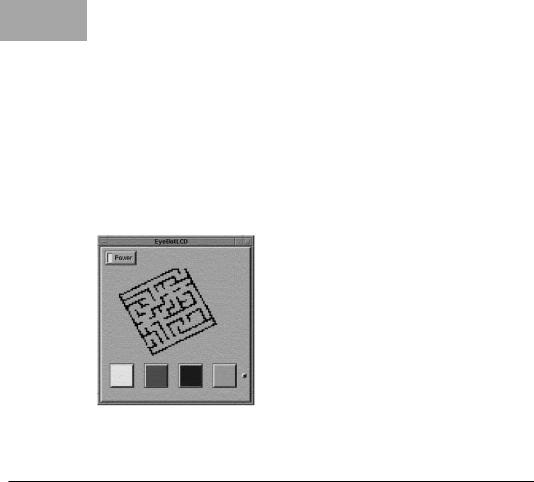
Figure 16.3 shows a downloaded screen shot of the robot’s on-board LCD after it finished exploring a maze environment and generated a configuration space map.

Figure 16.3: EyeBot screen shot

16.3 Boundary-Following Algorithm

When a robot encounters an obstacle, a boundary-following algorithm is activated, to ensure that all paths around the obstacle are checked. This will locate all possible paths to navigate around the obstacle.

In our approach, the robot follows the edge of an obstacle (or a wall) until it returns close to its starting position, thereby fully enclosing the obstacle. Keeping track of the robot’s exact position and orientation is crucial, because this may not only result in an imprecise map, but also lead to mapping the same obstacle twice or failing to return to an initial position. This task is non-trivial, since we work without a global positioning system and allow imperfect sensors.

Care is also taken to keep a minimum distance between robot and obstacle or wall. This should ensure the highest possible sensor accuracy, while avoiding a collision with the obstacle. If the robot were to collide, it would lose its position and orientation accuracy and may also end up in a location where its maneuverability is restricted.

Obstacles have to be stationary, but no assumptions are made about their size and shape. For example, we do not assume that obstacle edges are straight lines or that edges meet in rectangular corners. Due to this fact, the boundaryfollowing algorithm must take into account any variations in the shape and angle of corners and the curvature of obstacle surfaces.

232

Algorithm Execution

Path planning is required to allow the robot to reach a destination such as an unexplored area in the physical environment. Many approaches are available to calculate paths from existing maps. However, as in this case the robot is just in the process of generating a map, this limits the paths considered to areas that it has explored earlier. Thus, in the early stages, the generated map will be incomplete, possibly resulting in the robot taking sub-optimal paths.

Our approach relies on a path planning implementation that uses minimal map data like the DistBug algorithm [Kamon, Rivlin 1997] to perform path planning. The DistBug algorithm uses the direction toward a target to chart its course, rather than requiring a complete map. This allows the path planning algorithm to traverse through unexplored areas of the physical environment to reach its target. The algorithm is further improved by allowing the robot to choose its boundary-following direction freely when encountering an obstacle.

16.4 Algorithm Execution

A number of states are defined for each cell in the occupancy grid. In the beginning, each cell is set to the initial state “unknown”. Whenever a free space or an obstacle is encountered, this information is entered in the grid data structure, so cells can either be “free” or contain an “obstacle”. In addition we introduce the states “preliminary free” and “preliminary obstacle” to deal with sensor error and noise. These temporal states can later be either confirmed or changed when the robot passes within close proximity through that cell. The algorithm stops when the map generation is completed; that is, when no more preliminary states are in the grid data structure (after an initial environment scan).

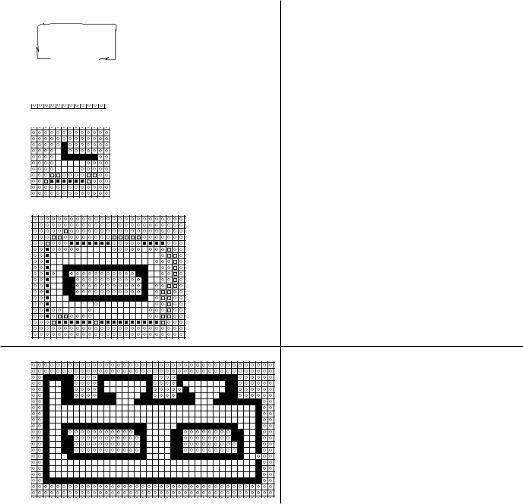
Our algorithm uses a rather coarse occupancy grid structure for keeping track of the space the robot has already visited, together with the much higherresolution configuration space to record all obstacles encountered. Figure 16.4 shows snapshots of pairs of grid and space during several steps of a map generation process.

In step A, the robot starts with a completely unknown occupancy grid and an empty corresponding configuration space (i.e. no obstacles). The first step is to do a 360° scan around the robot. For this, the robot performs a rotation on the spot. The angle the robot has to turn depends on the number and location of its range sensors. In our case the robot will rotate to +90° and –90°. Grid A shows a snapshot after the initial range scan. When a range sensor returns a

233

D

Figure 16.4: Stepwise environment exploration with corresponding occupancy grids and configuration spaces

value less than the maximum measurement range, then a preliminary obstacle is entered in the cell at the measured distance. All cells between this obstacle and the current robot position are marked as preliminary empty. The same is entered for all cells in line of a measurement that does not locate an obstacle; all other cells remain “unknown”. Only final obstacle states are entered into the configuration space, therefore space A is still empty.

In step B, the robot drives to the closest obstacle (here the wall toward the top of the page) in order to examine it closer. The robot performs a wallfollowing behavior around the obstacle and, while doing so, updates both grid and space. Now at close range, preliminary obstacle states have been changed to final obstacle states and their precise location has been entered into configuration space B.

234

Simulation Experiments

In step C, the robot has completely surrounded one object by performing the wall-following algorithm. The robot is now close again to its starting position. Since there are no preliminary cells left around this rectangular obstacle, the algorithm terminates the obstacle-following behavior and looks for the nearest preliminary obstacle.

In step D, the whole environment has been explored by the robot, and all preliminary states have been eliminated by a subsequent obstacle-following routine around the rectangular obstacle on the right-hand side. One can see the match between the final occupancy grid and the final configuration space.

16.5 Simulation Experiments

Experiments were conducted first using the EyeSim simulator (see Chapter 13), then later on the physical robot itself. Simulators are a valuable tool to test and debug the mapping algorithm in a controlled environment under various constraints, which are hard to maintain in a physical environment. In particular, we are able to employ several error models and error magnitudes for the robot sensors. However, simulations can never be a substitute for an experiment in a physical environment [Bernhardt, Albright 1993], [Donald 1989].

Collision detection and avoidance routines are of greater importance in the physical environment, since the robot relies on dead reckoning using wheel encoders for determining its exact position and orientation. A collision may cause wheel slippage, and therefore invalidate the robot’s position and orientation data.

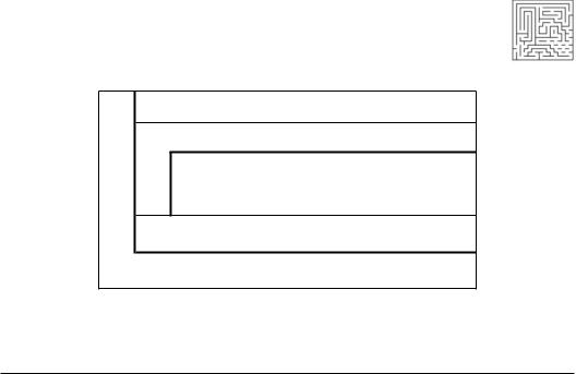
The first test of the mapping algorithm was performed using the EyeSim simulator. For this experiment, we used the world model shown in Figure 16.5

(a). Although this is a rather simple environment, it possesses all the required characteristic features to test our algorithm. The outer boundary surrounds two smaller rooms, while some other corners require sharp 180° turns during the boundary-following routine.

Figures 16.5 (b-d) show various maps that were generated for this environment. Varying error magnitudes were introduced to test our implementation of the map generation routine. From the results it can be seen that the configuration space representation gradually worsens with increasing error magnitude. Especially corners in the environment become less accurately defined. Nevertheless, the mapping system maintained the correct shape and structure even though errors were introduced.

We achieve a high level of fault tolerance by employing the following techniques:

•Controlling the robot to drive as close to an obstacle as possible.

•Limiting the error deviation of the infrared sensors.

•Selectively specifying which points are included in the map.

By limiting the points entered into the configuration space representation to critical points such as corners, we do not record any deviations along a straight

235

16 Map Generation

edge of an obstacle. This makes the mapping algorithm insensitive to small disturbances along straight lines. Furthermore, by maintaining a close distance to the obstacles while performing boundary-following, any sudden changes in sensor readings from the infrared sensors can be detected as errors and eliminated.

Figure 16.5: Simulation experiment:

(a) simulated environment (b) generated map with zero error model

(c)with 20% PSD error (d) with 10% PSD error and 5% positioning error

16.6Robot Experiments

Using a physical maze with removable walls, we set up several environments to test the performance of our map generation algorithm. The following figures show a photograph of the environment together with a measured map and the generated map after exploration through the robot.

Figure 16.6 represents a simple environment, which we used to test our map generation implementation. A comparison between the measured and generated map shows a good resemblance between the two maps.

Figure 16.7 displays a more complicated map, requiring more frequent turns by the robot. Again, both maps show the same shape, although the angles are not as closely mapped as in the previous example.

The final environment in Figure 16.8 contains non-rectangular walls. This tests the algorithm’s ability to generate a map in an environment without the assumption of right angles. Again, the generated maps show distinct shape similarities.

236