

Advanced Probability Theory for Biomedical Engineers - John D. Enderle
.pdfTRANSFORMATIONS OF RANDOM VARIABLES 53
Drill Problem 6.1.3. Random variable x has the PDF
fx (α) = 0.5α(u(α) − u(α − 2)).
Random variable z is defined by |
|
−1, |
x ≤ 0.5 |
z = x + 0.5, |
0.5 < x ≤ 1 |
3, |
x > 1. |
Determine: (a) Fz(−1), (b)Fz(0), (c )Fz(3/2), (d )Fz(4).
Answers: 1/4, 1/16, 1/16, 1.
Drill Problem 6.1.4. Random variable x has PDF
fx (α) = e −α−1u(α + 1).
Random variable z = 1/x2 . Determine: (a) Fz(1/8), (b)Fz(1/2), (c )Fz(4), (d ) fz(4).
Answers: 0.0519, 0.617, 0.089, 0.022.
6.2UNIVARIATE PDF TECHNIQUE
The previous section solved the problem of determining the probability distribution of a function of a random variable using the cumulative distribution function. Now, we introduce a second method for calculating the probability distribution of a function z = g (x) using the probability density function, called the PDF technique. The PDF technique, however, is only applicable for functions of random variables in which z = g (x) is continuous and does not equal a constant in any interval in which fx is nonzero. We introduce the PDF technique for two reasons. First, in many situations it is much simpler to use than the CDF technique. Second, we will find the PDF method most useful in extensions to multivariate functions. In this section, we discuss a wide variety of situations using the PDF technique with functions of continuous random variables. Then, a method for handling mixed random variables with the PDF technique is introduced. Finally, we consider computing the conditional PDF of a function of a random variable using the PDF technique.
6.2.1Continuous Random Variable
Theorem 6.2.1. Let x be a continuous RV with PDF fx (α) and let the RV z = g (x) . Assume g is continuous and not constant over any interval for which fx = 0 . Let
αi = αi (γ ) = g −1(γ ), i = 1, 2, . . . , |
(6.11) |

54 ADVANCED PROBABILITY THEORY FOR BIOMEDICAL ENGINEERS
denote the distinct solutions to g (αi ) = γ . Then |
|
|
|
∞ |
fx (αi (γ )) |
|
|
fz(γ ) = i=1 |
|
, |
(6.12) |
|g (1)(αi (γ ))| |
|||
where we interpret
fx (αi (γ )) = 0, |g (1)(αi (γ ))|
if fx (αi (γ ) = 0.
Proof. Let h > 0 and define
I (γ , h) = {x : γ − h < g (x) ≤ γ }.
Partition I (γ , h) into disjoint intervals of the form
Ii (γ , h) = (ai (γ , h), bi (γ , h)), i = 1, 2, . . . ,
such that
|
|
|
|
|
|
|
|
|
∞ |
|
|
|
|
|
|
|
|
|
|
|
|
I (γ , h) = Ii (γ , h). |
|
|
|
|
|
|
|||||||
|
|
|
|
|
|
|
|
i=1 |
|
|
|
|
|
|
|
|
|
Then |
|
|
|
|
|
|
|
|
|
|
|
|
|
|
|
|
|
|
Fz(γ ) − Fz(γ − h) = |
∞ |
(Fx (bi (γ , h)) − Fx (ai (γ , h))) |
|
|||||||||||||
|
|
|
|||||||||||||||
|
|
|
|
|
|
|
i=1 |
|
|
|
|
|
|
|
|
|
|
By hypothesis, |
|
|
|
h) = h 0 bi |
|
h) = |
|
|
|
|
|
|
|||||
|
h 0 ai ( |
|
(γ , |
i ( |
|
) |
|
|
|
||||||||
|
lim |
|
γ , |
|
|
lim |
|
α |
γ |
|
. |
|
|
||||
|
|
→ |
|
|
|
|
|
→ |
|
|
|
|
|
|
|
|
|
Note that (for all γ with fx (αi (γ )) = 0) |
|
|
|
|
|
|
|
|
|
|
|
||||||
lim |
bi (γ , h) − ai (γ , h) |
|
lim |
|
|
bi (γ , h) − ai (γ , h) |
|
|
1 |
, |
|||||||
|
|
|
|
|
|
|
|g (1)(αi (γ ))| |
||||||||||
h→0 |
h |
|
= h→0 |g (bi (γ , h)) − g (ai (γ , h))| = |
|
|||||||||||||
and that
lim Fx (bi (γ , h)) − Fx (ai (γ , h)) = fx (αi (γ )). h→0 bi (γ , h) − ai (γ , h)
The desired result follows by taking the product of the above limits. The absolute value ap-
pears because by construction we have bi > ai |
and h > 0, whereas g (1) may be positive or |
negative. |
|

TRANSFORMATIONS OF RANDOM VARIABLES 55
Example 6.2.1. Random variable x is uniformly distributed in the interval 0–4. Find the PDF for random variable z = g (x) = 2x + 1.
Solution. In this case, there is only one solution to the equation γ = 2α + 1, given by α1 = (γ − 1)/2. We easily find g (1)(α) = 2. Hence
fz(γ ) = fx ((γ − 1)/2)/2 = |
1/8, |
1 < γ < 9 |
|
0, |
otherwise. |
|
Example 6.2.2. Random variable x has PDF
fx (α) = 0.75(1 − α2)(u(α + 1) − u(α − 1)).
Find the PDF for random variable z = g (x) = 1/x2.
Solution. For γ < 0, there are no solutions to g (αi ) = γ , so that fz(γ ) = 0 for γ < 0. For γ > 0 there are two solutions to g (αi ) = γ :
1 |
|
and |
1 |
|
||
α1(γ ) = − √ |
|
, |
α2(γ ) = √ |
|
. |
|
γ |
γ |
|||||
Since γ = g (α) = α−2, we have g (1)(α) = −2α−3; hence, |g (1)(αi )| = 2/|αi |3 = 2|γ |3/2, and
|
|
|
|
|
|
fz( |
γ |
) = |
fx (−γ −1/2) + fx (γ −1/2) |
u( |
γ |
. |
|
|
|
|
|
|
|
|
|
|
|
|
|
|
|
|
|
|
|
|
|||||||
|
|
|
|
|
|
|
2γ 3/2 |
|
) |
|
|
|
|
|
|
|
|||
Substituting, |
|
|
|
|
|
|
|
|
|
|
|
|
|
|
|
|
|
|
|
fz( |
γ |
) = |
|
0.75(1 − γ −1)(u(1 − γ −1/2) − 0 + 1 − u(γ −1/2 − 1)) |
u( |
γ |
. |
||||||||||||
|
|
||||||||||||||||||
|
|
|
|
|
|
2γ 3/2 |
|
|
|
|
|
|
) |
|
|||||
Simplifying, |
|
|
|
|
|
|
|
|
|
|
|
|
|
|
|
|
|
|
|
|
|
fz( |
γ |
) = |
0.75(1 − γ −1)(u(γ − 1) − 0 + 1 − u(1 − γ )) |
u( |
γ |
) |
, |
|
|
||||||||
|
|
|
|
|
|||||||||||||||
|
|
|
|
|
|
2γ 3/2 |
|
|
|
|
|
|
|
|
|||||
or |
|
|
|
|
|
|
|
|
|
|
|
|
|
|
|
|
|
|
|
|
|
|
|
|
|
|
|
|
3 |
5 |
|
|
|
|
|
|
|
|
|
|
|
|
|
|
|
fz(γ ) = 0.75(γ − 2 − γ |
− 2 )u(γ − 1). |
|
|
|
|
|
|
||||||
Example 6.2.3. Random variable x has PDF
fx (α) = 16 (1 + α2)(u(α + 1) − u(α − 2)).
Find the PDF for random variable z = g (x) = x2.

56 ADVANCED PROBABILITY THEORY FOR BIOMEDICAL ENGINEERS
Solution. For γ < 0 there are no solutions to g (αi ) = γ , so that fz(γ ) = 0 for γ < 0. For γ > 0 there are two solutions to g (αi ) = γ :
α1(γ ) = −√γ , and α2(γ ) = √γ .
Since γ = g (α) = α2, we have g (1)(α) = 2α; hence, |g (1)(αi )| = 2|αi | = 2√γ , and
|
|
|
|
|
|
|
|
|
|
|
|
fx (−√ |
|
) + fx (√ |
|
) |
|
|
|
|
|
|
|
|
|
|
|||||||||||
|
|
|
|
|
|
|
fz(γ ) = |
γ |
γ |
u(γ ). |
|
|
|
|
|
|
|
||||||||||||||||||||
|
|
|
|
|
|
|
|
|
|
|
2√ |
|
|
|
|
|
|
|
|
|
|
|
|
|
|
|
|||||||||||
|
|
|
|
|
|
|
|
|
|
|
γ |
|
|
|
|
|
|
|
|
|
|
|
|
||||||||||||||
Substituting, |
|
|
|
|
|
|
|
|
|
|
|
|
|
|
|
|
|
|
|
|
|
|
|
|
|
|
|
|
|
|
|
|
|
|
|
|
|
|
(γ ) |
|
1 + γ |
( |
(1 |
|
√ |
|
) |
( |
|
2 |
|
|
√ |
|
) |
|
(√ |
|
|
1) |
|
(√ |
|
|
2)) |
|
(γ ). |
||||||||
|
|
|
γ |
|
|
|
γ |
|
γ |
|
|
γ |
|
|
|||||||||||||||||||||||
fz |
|
= |
12√ |
γ |
u |
|
− |
|
|
|
− u |
− |
|
− |
|
|
|
|
|
|
+ u |
|
|
|
|
|
+ |
|
− u |
|
|
− |
|
u |
|
||
Simplifying,
1 + γ
fz(γ ) = 12√γ (u(1 − γ ) − 0 + 1 − u(γ − 4))u(γ ),
or
(γ −1/2 + γ 1/2)/6, |
0 < γ < 1 |
|
fz(γ ) = (γ −1/2 + γ 1/2)/12, |
1 < γ < 4 |
|
0, |
elsewhere. |
6.2.2Mixed Random Variable
Consider the problem where random variable x is mixed, and we wish to find the PDF for z = g (x). Here, we treat the discrete and continuous portions of fx separately, and then combine the results to yield fz. The continuous part of the PDF of x is handled by the PDF technique. To illustrate the use of this technique, consider the following example.
Example 6.2.4. Random variable x has PDF |
|
|
|
|
|
|
|
|||
|
3 |
|
|
|
1 |
|
1 |
|
||
fx (α) = |
|
(u(α + 1) |
− u(α − 1)) |
+ |
|
δ(α + 0.5) |
+ |
|
|
δ(α − 0.5). |
8 |
8 |
8 |
||||||||
Find the PDF for the RV z = g (x) = e −x .
Solution. There is only one solution to g (α) = γ :
α1(γ ) = − ln(γ ).
We have g (1)(α1) = −e ln(γ ) = −γ . The probability masses of 1/8 for x at −0.5 and 0.5 are mapped to probability masses of 1/8 for z at e 0.5 and e −0.5, respectively. For all γ > 0 such that

TRANSFORMATIONS OF RANDOM VARIABLES 57
|α1(γ ) ± 0.5| > 0 we have
fz(γ ) = fx (− ln(γ )) .
γ
Combining these results, we find
|
3 |
|
1 |
1 |
|
||
fz(γ ) = |
|
(u(γ − e −1) − u(γ − e )) + |
|
δ(γ − e 0.5) + |
|
δ(γ − e −0.5). |
|
8γ |
8 |
8 |
|||||
6.2.3Conditional PDF Technique
Since a conditional PDF is also a PDF, the above techniques apply to find the conditional PDF for z = g (x), given event A. Consider the problem where random variable x has PDF fx , and we wish to evaluate the conditional PDF for random variable z = g (x), given that event A occurred. Depending on whether the event A is defined on the range or domain of z = g (x), one of the following two methods may be used to determine the conditional PDF of z using the PDF technique.
(i)If A is an event defined for an interval on z, the conditional PDF, fz| A, is computed by first evaluating fz using the technique in this section. Then, by the definition of a conditional PDF, we have
fz| A(γ | A) = |
fz(γ ) |
γ A, |
(6.13) |
P (A) , |
and fz| A(γ | A) = 0 for γ A.
(ii)If A is an event defined for an interval on x, we will use the conditional PDF of x to evaluate the conditional PDF for z as
fz| A( |
γ |
∞ |
fz| A(αi (γ )| A) |
. |
|
|
| A) = i=1 |g (1)(αi (γ ))| |
(6.14) |
|||
Example 6.2.5. Random variable x has the PDF
fx (α) = 16 (1 + α2)(u(α + 1) − u(α − 2)).
Find the PDF for random variable z = g (x) = x2, given A = {x : x > 0}.
Solution. First, we solve for the conditional PDF for x and then find the conditional PDF for z, based on fx| A. We have
|
1 |
|
2 |
7 |
|
P (A) = |
|
(1 + α2)d α = |
|||
|
|
|
, |
||
6 |
0 |
9 |
|||

58 ADVANCED PROBABILITY THEORY FOR BIOMEDICAL ENGINEERS
so that
fx| A(α| A) = 143 (1 + α2)(u(α) − u(α − 2)).
There is only one solution to γ = g (α) = α2 on the interval 0 < α < 2 where fx| A = 0. We |
|||||||||||||
have α1(γ ) = |
√ |
|
and |g (1)(α1(γ ))| = 2√ |
|
|
. Consequently, |
|
|
|||||
γ |
γ |
|
|
||||||||||
|
3 |
√ |
|
1 |
|
|
|
||||||
|
|
|
fz| A(γ | A) = |
|
γ |
+ √ |
|
(u(γ ) |
− u(γ − 4)). |
|
|||
|
|
|
28 |
||||||||||
|
|
|
γ |
||||||||||
Drill Problem 6.2.1. Random variable x has a uniform PDF in the interval 0–8. Random variable z = 3x + 1 .Use the PDF method to determine: (a) fz(0), (b) fz(6), (c )E(z), (d )σz2.
Answers: 13, 48, 0, 1/24.
Drill Problem 6.2.2. Random variable x has the PDF
9α2, |
0 ≤ α < 0.5 |
fx (α) = 3(1 − α2), |
0.5 ≤ α ≤ 1 |
0, |
otherwise. |
Random variable z = x3 .Use the PDF method to determine: (a) fz(1/27), (b) fz(1/4), (c ) fz|z>1/8
(1/4|z > 1/8), (d ) fz(2).
Answers: 1.52, 0, 3, 2.43.
Drill Problem 6.2.3. Random variable x has the PDF
2
fx (α) = 9 α(u(α) − u(α − 3)).
Random variable z = (x − 1)2. Use the PDF method to determine: (a) fz(1/4), (b) fz(9/4), (c ) fz|z≤1 (1/4|z ≤ 1), (d )E(z|z ≤ 1).
Answers: 4/9, 5/27, 1/3, 1.
Drill Problem 6.2.4. Random variable x has the PDF
2
fx (α) = 9 (α + 1)(u(α + 1) − u(α − 2)).
Random variable z = 2x2 and event A = {x : x ≥ 0}. Determine: (a) P (A), (b) fx| A (1| A), (c ) fz| A(2| A),(d ) fz| A(9| A).
Answers: 0, 1/2, 1/8, 8/9.

TRANSFORMATIONS OF RANDOM VARIABLES 59
6.3ONE FUNCTION OF TWO RANDOM VARIABLES
Consider a random variable z = g (x, y) created from jointly distributed random variables x and y. In this section, the probability distribution of z = g (x, y) is computed using a CDF technique similar to the one at the start of this chapter. Because we are dealing with regions in a plane instead of intervals on a line, these problems are not as straightforward and tractable as before.
With z = g (x, y), we have |
|
|
Fz(γ ) = P (z ≤ γ ) = P (g (x, y) ≤ γ ) = P ((x, y) A(γ )), |
(6.15) |
|
where |
|
|
A(γ ) = {(x, y) : g (x, y) ≤ γ }. |
(6.16) |
|
The CDF for the RV z can then be found by evaluating the integral |
|
|
Fz(γ ) = |
A(γ ) dFx,y (α, β). |
(6.17) |
This result cannot be continued further until a specific Fx,y and g (x, y) are considered. Remember that in the case of a single random variable, our efforts primarily dealt with algebraic manipulations. Here, our efforts are concentrated on evaluating Fz through integrals, with the ease of solution critically dependent on g (x, y).
The ease in solution for Fz is dependent on transforming A(γ ) into proper limits of integration. Sketching the support region for fx,y (the region where fx,y = 0, or Fx,y is not constant) and the region A(γ ) is often most helpful, even crucial, in the problem solution. Pay careful attention to the limits of integration to determine the range of integration in which the integrand is zero because fx,y = 0. Let us consider several examples to illustrate the mechanics of the CDF technique and also to provide further insight.
Example 6.3.1. Random variables x and y have joint PDF
fx,y (α, β) = |
1/4, |
0 < α < 2, 0 < β < 2 |
0, |
otherwise. |
Find the CDF for z = x + y.
Solution. We have A(γ ) = {(α, β) : α + β ≤ γ }. We require the volume under the surface fx,y (α, β) where α ≤ γ − β:
∞ |
γ −β |
Fz(γ ) = |
fx,y (α, β)d α dβ. |
−∞ |
−∞ |

60 ADVANCED PROBABILITY THEORY FOR BIOMEDICAL ENGINEERS
|
|
|
|
γ |
β |
|
|
|
|
|
|
|
|
|
|
|
|
|
β |
|
|
|
|
|
|
|
2 |
|
|
|
2 |
|
|
|
|
γ |
|
|
|
γ − 2 |
|
|
|
|
|
|
|
|
|
|
|
|
|
0 |
γ |
2 |
α |
0 |
γ −2 |
2 |
γ |
α |
|
( a ) 0 < γ < 2 |
|
|
( b ) 2 < γ < 4 |
|
|
||
FIGURE 6.3: Plots for Example 6.3.1.
For γ < 0 we have Fz(γ ) = 0. For 0 ≤ γ < 2, with the aid of Figure 6.3(a) we obtain
2 |
γ −β 1 |
1 |
γ 2. |
|||
Fz(γ ) = 0 0 |
|
|
d αdβ = |
|
|
|
|
4 |
8 |
||||
For 2 ≤ γ < 4, referring to Figure 6.3(b), we consider the complementary region (to save some work):
Fz(γ ) = 1 − |
2 |
2 |
1 |
d αdβ = 1 |
|
1 |
(4 |
− γ )2. |
|
|
|
− |
|||||||
γ −2 γ −β |
|
|
|
||||||
4 |
8 |
||||||||
Finally, for 4 ≤ γ , Fz(γ ) = 1.
Example 6.3.2. Random variables x and y have joint PDF
fx,y (α, β) = |
1, |
0 < α < 1, 0 < β < 1 |
0, |
otherwise. |
Find the PDF for z = x − y.
Solution. We have A(γ ) = {(α, β) : α − β ≤ γ }. We require the volume under the surface fx,y (α, β) where α ≤ γ + β:
∞γ +β
Fz(γ ) = |
fx,y (α, β)d αdβ. |
−∞ |
−∞ |
For γ < −1 we have Fz(γ ) = 0 and fz(γ ) = 0. With the aid of Figure 6.4(a), for −1 ≤ γ < 0,
1 |
γ +β |
1 |
|
+ γ )2, |
Fz(γ ) = |
d αdβ = |
|
(1 |
|
2 |
||||
−γ |
0 |
|
|
|

|
|
|
|
|
|
|
TRANSFORMATIONS OF RANDOM VARIABLES 61 |
||||||
1 |
|
|
|
β |
1 |
|
|
β |
|
|
|
||
|
|
|
|
|
|||||||||
|
|
|
|
|
|
|
|
|
|
|
|
||
|
|
|
|
|
|
|
|
|
|
|
|
||
−γ |
|
|
|
|
|
|
1− γ |
|
|
|
|
|
|
|
|
|
|
|
|
|
|
|
|
|
|
||
0 |
|
|
|
|
|
|
0 |
|
|
|
|
|
|
|
|
|
|
|
|
|
|
|
|
|
|
||
|
|
|
1 + γ 1 α |
|
|
γ |
1 α |
|
|||||
|
|
|
|
(a) −1 < γ < 0 |
|
|
|
(b) 0 < γ < 1 |
|||||
FIGURE 6.4: Plots for Example 6.3.2.
so that fz(γ ) = 1 + γ . For 0 ≤ γ < 1, we consider the complementary region shown in Figure 6.4(b) (to save some work):
1−γ |
1 |
1 |
(1 − γ )2, |
|
|
Fz(γ ) = 1 − |
|
d αdβ = 1 − |
|
|
|
γ +β |
2 |
|
|||
0 |
|
|
|
|
|
so that fz(γ ) = 1 − γ . Finally, for 1 ≤ γ , Fz(γ ) = 1, so that fz(γ ) = 0. |
|||||
Example 6.3.3. Find the CDF for z = x/y, where x and y have the joint PDF |
|
||||
fx,y (α, β) = |
1/α, |
0 < β < α < 1 |
|
||
0, |
otherwise. |
|
|||
Solution. We have A(γ ) = {(α, β) : α/β ≤ γ }. Inside the support region for fx,y , we have α/β > 1; hence, for γ < 1 we have Fz(γ ) = 0. As shown in Figure 6.5 it is easiest to integrate with respect to β first: for 1 ≤ γ ,
Fz(γ ) = |
1 |
α |
1 |
= 1 − |
0 |
α/γ α dβd α |
|||
|
β |
|
|
|
1 |
|
|
|
|
1 |
|
|
|
|
γ |
|
|
|
|
0 |
|
|
1 |
α |
1 |
. |
|
|
γ |
|
||
|
FIGURE 6.5: Integration region for Example 6.3.3.
62 ADVANCED PROBABILITY THEORY FOR BIOMEDICAL ENGINEERS
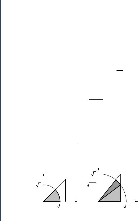
Example 6.3.4. Find the CDF for z = x2 + y2, where x and y have the joint PDF
fx,y (α, β) = |
3α, |
0 < β < α < 1 |
0, |
otherwise. |
Solution. We have A(γ ) = {(α, β) : α2 + β2 ≤ γ }. For γ < 0, we obtain Fz(γ ) = 0. Transforming to polar coordinates: α = r cos(θ ), β = r sin(θ ),
Fz(γ ) = |
|
2π |
|
fx,y (r cos(θ ), r sin(θ ))r dr d θ . |
||||
0 |
r 2≤γ |
|||||||
Referring to Figure 6.6(a), for 0 ≤ γ < 1, |
|
|
|
|
|
|||
|
|
π/4 |
√ |
|
|
1 |
|
|
|
|
γ |
3r 2 cos(θ )dr d θ = |
3 |
||||
Fz(γ ) = |
|
|
|
|
||||
|
|
|
|
√ |
|
γ 2 . |
||
|
0 |
0 |
|
2 |
||||
For 1 ≤ γ < 2, we split the integral into two parts: one with polar coordinates, the other using rectangular coordinates. With
|
|
|
|
|
|
|
|
|
|
√ |
|
|
|
|
|
|
|
|
|
|
|
|
θ |
|
|
|
γ − 1 |
, |
|
|
|
||||
|
|
|
|
|
|
|
|
|
|
||||||||
|
|
|
|
|
sin( |
|
1) = |
|
√ |
γ |
|
|
|
|
|
||
we find with the aid of Figure 6.6(b) that |
|
|
|
|
|
|
|
|
|
|
|
|
|||||
|
π/4 |
|
√ |
|
|
|
|
|
|
|
|
|
|
1 |
α√ |
|
|
|
|
|
|
|
|
|
|
|
|
|
|
γ −1 |
|||||
|
|
γ |
3r 2 cos(θ )dr d θ + |
||||||||||||||
Fz(γ ) = |
θ1 |
0 |
|
|
0 0 |
|
|
3αdβ d α, |
|||||||||
or |
|
|
|
|
|
|
|
|
|
|
|
|
|
|
|
|
|
|
|
|
|
|
|
|
1 |
|
3 |
|
|
|
3 |
|
|
|
|
|
|
Fz(γ ) = |
√ |
|
γ 2 − (γ − 1) 2 . |
|
|
|
|||||||||
|
|
2 |
|
|
|
||||||||||||
Finally, we have Fz(γ ) = 1 for 2 ≤ γ .
|
|
|
β |
|
|
γ |
|
|
β |
|
|
|
|
||||
|
|
|
|
|
|
|
|
|
|
|
|||||||
|
|
|
|
|
|
|
|
|
|
|
|
|
|||||
|
|
|
|
|
|
|
|
|
|
|
|
|
|||||
1 |
|
|
|
|
|
|
|
|
1 |
|
|
|
|
|
|
|
|
|
|
|
|
|
|
|
|
|
|
|
|
|
|
|
|
||
γ |
|
|
|
|
|
|
|
|
γ −1 |
|
|
|
|
|
|
|
|
|
|
|
|
|
|
|
|
|
|
|
|
|
|
|
|
||
0 |
|
|
|
|
|
|
|
0 |
|
|
|
|
|
|
|
|
|
|
|
|
|
|
|
|
|
|
|
|
|
|
|
|
|
||
|
|
γ 1 |
α |
1 |
γ |
α |
|||||||||||
|
|
|
|
|
|
|
|
||||||||||
|
|
|
(a) 0 < γ < 1 |
|
|
|
|
(b) 1 < γ < 2 |
|
|
|
|
|||||
FIGURE 6.6: Integration regions for Example 6.3.4.