


Basic Concepts of Pinch Analysis
Most industrial processes involve transfer of heat either from one process stream to another process stream (interchanging) or from a utility stream to a process stream. In the present energy crisis scenario all over the world, the target in any industrial process design is to maximize the process-to- process heat recovery and to minimize the utility (energy) requirements. To meet the goal of maximum energy recovery or minimum energy requirement (MER) an appropriate heat exchanger network (HEN) is required. The design of such a network is not an easy task considering the fact that most processes involve a large number of process and utility streams. As explained in the previous section, the traditional design approach has resulted in networks with high capital and utility costs. With the advent of pinch analysis concepts, the network design has become very systematic and methodical.
A summary of the key concepts, their significance, and the nomenclature used in pinch analysis is given below:
∙Combined (Hot and Cold ) Composite Curves: Used to predict targets for
∙Minimum energy (both hot and cold utility) required,
∙Minimum network area required, and
∙Minimum number of exchanger units required.
∙DTmin and Pinch Point : The DTmin value determines how closely the hot and cold composite curves can be ‘pinched’ (or squeezed) without violating the Second Law of Thermodynamics (none of the heat exchangers can have a temperature crossover).
∙Grand Composite Curve: Used to select appropriate levels of utilities (maximize cheaper utilities) to meet over all energy requirements.
∙Energy and Capital Cost Targeting : Used to calculate total annual cost of utilities and capital cost of heat exchanger network.
∙Total Cost Targeting: Used to determine the optimum level of heat recovery or the optimum DTmin value, by balancing energy and capital costs. Using this method, it is possible to obtain an accurate estimate (within 10 - 15%) of overall heat recovery system costs without having to design the system. The essence of the pinch approach is the speed of economic evaluation.
∙Plus/Minus and Appropriate Placement Principles: The “Plus/Minus” Principles provide guidance regarding how a process can be modified in order to reduce associated utility needs and costs. The Appropriate Placement Principles provide insights for proper integration of key equipments like distillation columns, evaporators, furnaces, heat engines, heat pumps etc. in order to reduce the utility requirements of the combined system.

∙Total Site Analysis : This concept enables the analysis of the energy usage for an entire plant site that consists of several processes served by a central utility system.
With further research, new topics like ‘Regional Energy Analysis’, ‘Network Pinch’, ‘Top Level Analysis’, ‘Optimisation of Combined Heat & Power’, ‘Water Pinch’, ‘Hydrogen Pinch’ etc. Are being developed. These pinch concepts are discussed in Section-3 and 5. These basic terms and concepts have become the foundation of what we now call Pinch Technology.
Steps of Pinch Analysis
In any Pinch Analysis problem, whether a new project or a retrofit situation, a well-defined stepwise procedure is followed (Figure 3). It should be noted that these steps are not necessarily performed on a once-through basis, independent of one another. Additional activities such as resimulation and data modification occur as the analysis proceeds and some iteration between the various steps is always required.
Figure 3: Steps of Pinch Analysis
1.Identification of the Hot, Cold and Utility Streams in the Process
∙‘Hot Streams’ are those that must be cooled or are available to be cooled. e.g. product cooling before storage
∙‘Cold Streams’ are those that must be heated e.g. feed preheat before a reactor.
∙‘Utility Streams’ are used to heat or cool process streams, when heat exchange between process streams is not practical or economic. A number of different hot utilities (steam,
hot water, flue gas, etc.) and cold utilities (cooling water, air, refrigerant, etc.) are used in industry.

The identification of streams needs to be done with care as sometimes, despite undergoing changes in temperature, the stream is not available for heat exchange. For example, when a gas stream is compressed the stream temperature rises because of the conversion of mechanical energy into heat and not by any fluid to fluid heat exchange. Hence such a stream may not be available to take part in any heat exchange. In the context of pinch analysis, this stream may or may not be considered to be a process stream.
2.Thermal Data Extraction for Process & Utility Streams
For each hot, cold and utility stream identified, the following thermal data is extracted from the process material and heat balance flow sheet:
∙Supply temperature (TS oC) : the temperature at which the stream is available.
∙Target temperature (TT oC) : the temperature the stream must be taken to.
∙Heat capacity flow rate (CP kW/ oC) : the product of flow rate (m) in kg/sec and specific heat (Cp kJ/kg 0C).
CP = m x Cp
∙Enthalpy Change ( H) associated with a stream passing through the exchanger is given by the First Law of Thermodynamics:
First Law energy equation: H = Q ± W
In a heat exchanger, no mechanical work is being performed:
W = 0 (zero)
The above equation simplifies to: H = Q, where Q represents the heat supply or demand associated with the stream. It is given by the relationship: Q= CP x (TS - TT).
Enthalpy Change, H = CP x (TS - TT)
** Here the specific heat values have been assumed to be temperature independent within the operating range.
The stream data and their potential effect on the conclusions of a pinch analysis should be considered during all steps of the analysis. Any erroneous or incorrect data can lead to false conclusions. In order to avoid mistakes, the data extraction is based on certain qualified principles. For details on principles of data extraction, check out Link-2 at the end of the article. The data extracted is presented in Table 1.

TABLE 1: TYPICAL STREAM DATA
STREAM |
|
STREAM |
|
SUPPLY |
|
TARGET |
|
HEAT |
|
ENTH. CHANGE |
NUMBER |
|
NAME |
|
TEMP. |
|
TEMP. |
|
CAP. FLOW. |
|
kW |
|
|
|
°C |
|
|
|||||
|
|
|
|
°C |
|
|
kW /°C |
|
|
|
|
|
|
|
|
|
|
|
|
||
|
|
|
|
|
|
|
|
|
|
|
|
|
|
|
|
|
|
|
|
|
|
1 |
|
FEED |
|
60 |
|
205 |
|
20 |
|
2900 |
|
|
|
|
|
|
|
|
|
|
|
|
|
|
|
|
|
|
||||
2 |
|
REAC.OUT |
|
270 |
|
160 |
|
18 |
|
1980 |
|
|
|
|
|
|
|
|
|
|
|
|
|
|
|
|
|
|
||||
3 |
|
PRODUCT |
|
220 |
|
70 |
|
35 |
|
5250 |
|
|
|
|
|
|
|
|
|
|
|
|
|
|
|
|
|
|
||||
4 |
|
RECYCLE |
|
160 |
|
210 |
|
50 |
|
2500 |
|
|
|
|
|
|
|
|
|
|
|
3. Selection of Initial DTmin value
The design of any heat transfer equipment must always adhere to the Second Law of Thermodynamics that prohibits any temperature crossover between the hot and the cold stream i.e. a minimum heat transfer driving force must always be allowed for a feasible heat transfer design. Thus the temperature of the hot and cold streams at any point in the exchanger must always have a minimum temperature difference (DTmin). This DTmin value represents the bottleneck in the heat recovery.
In mathematical terms, at any point in the exchanger

 Hot stream Temp. ( TH ) ( TC ) Cold stream Temp. DTmin

The value of DTmin is determined by the overall heat transfer coefficients (U) and the geometry of the heat exchanger. In a network design, the type of heat exchanger to be used at the pinch will determine the practical Dtmin for the network. For example, an initial selection for the Dtmin value for shell and tubes may be 3-5 0C (at best) while compact exchangers such as plate and frame often allow for an initial selection of 2-3 0C. The heat transfer equation, which relates Q, U, A and LMTD (Log Mean Temperature Difference) is depicted in Figure 4.
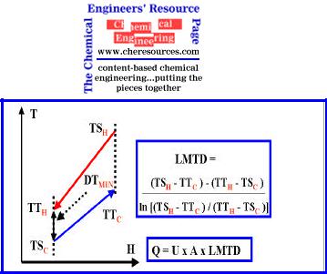
Figure 4: Heat Transfer Equation
For a given value of heat transfer load (Q), if smaller values of DTmin are chosen, the area requirements rise. If a higher value of DTmin is selected the heat recovery in the exchanger decreases and demand for external utilities increases. Thus, the selection of DTmin value has implications for both capital and energy costs. This concept will become clearer with the help of composite curves and total cost targeting discussed later.
Just as for a single heat exchanger, the choice of DTmin (or approach temperature) is vital in the design of a heat exchanger networks. To begin the process an initial DTmin value is chosen and pinch analysis is carried out. Typical DTmin values based on experience are available in literature for reference. A few values based on Linnoff March’s application experience are tabulated below for shell and tube heat exchangers.
|
|
|
No |
Industrial Sector |
Experience DTmin |
|
|
Values |
|
|
|
|
|
|
1 |
Oil Refining |
20-40ºC |
|
|
|
|
|
|
2 |
Petrochemical |
10-20ºC |
|
|
|
|
|
|
3 |
Chemical |
10-20ºC |
|
|
|
|
|
|
4 |
Low Temperature |
3-5ºC |
|
Processes |
|
|
|
|
|
|
|
For more details on typical DTmin values, check Link-3 at the end of the article.
4. Construction of Composite Curves and Grand Composite Curve
∙COMPOSITE CURVES : Temperature - Enthalpy (T - H) plots known as ‘Composite curves’ have been used for many years to set energy targets ahead of design. Composite curves consist of temperature (T) – enthalpy (H) profiles of heat availability in the process (the hot composite curve) and heat demands in the process (the cold composite curve) together in a graphical representation.
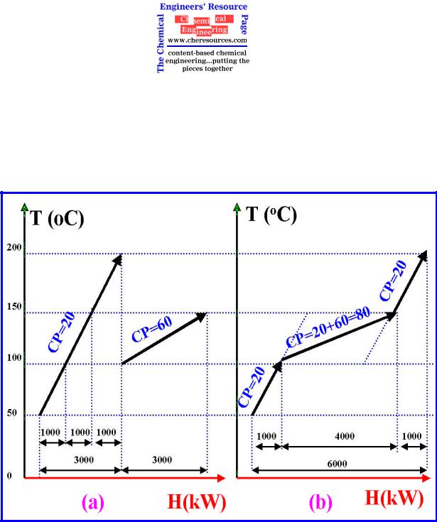
In general any stream with a constant heat capacity (CP) value is represented on a T - H diagram by a straight line running from stream supply temperature to stream target temperature. When there are a number of hot and cold streams, the construction of hot and cold composite curves simply involves the addition of the enthalpy changes of the streams in the respective temperature intervals. An example of hot composite curve construction is shown in Figure 5(a) and (b). A complete hot or cold composite curve consists of a series of connected straight lines, each change in slope represents a change in overall hot stream heat capacity flow rate (CP).
Figure 5: Temperature-Enthalpy Relations Used to Construct Composite Curves
For heat exchange to occur from the hot stream to the cold stream, the hot stream cooling curve must lie above the cold stream-heating curve. Because of the ‘kinked’ nature of the composite curves (Figure 6), they approach each other most closely at one point defined as the minimum approach temperature (DTmin). DTmin can be measured directly from the T-H profiles as being the minimum vertical difference between the hot and cold curves. This point of minimum temperature difference represents a bottleneck in heat recovery and is commonly referred to as the "Pinch". Increasing the DTmin value results in shifting the of

the curves horizontally apart resulting in lower process to process heat exchange and higher utility requirements. At a particular DTmin value, the overlap shows the maximum possible scope for heat recovery within the process. The hot end and cold end overshoots indicate minimum hot utility requirement (QHmin) and minimum cold utility requirement (QCmin), of the process for the chosen DTmin.
Thus, the energy requirement for a process is supplied via process to process heat exchange and/or exchange with several utility levels (steam levels, refrigeration levels, hot oil circuit, furnace flue gas, etc.).
Graphical constructions are not the most convenient means of determining energy needs. A numerical approach called the "Problem Table Algorithm" (PTA) was developed by Linnhoff & Flower (1978) as a means of determining the utility needs of a process and the location of the process pinch. The PTA lends itself to hand calculations of the energy targets. For more details on PTA see Link-4 at the end of the article.
To summarize, the composite curves provide overall energy targets but do not clearly indicate how much energy must be supplied by different utility levels. The utility mix is determined by the Grand Composite Curve.
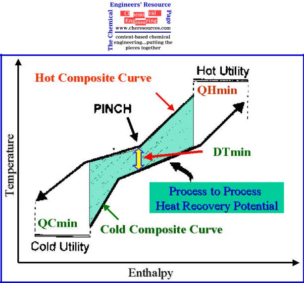
Figure 6: Combined Composite Curves
∙GRAND COMPOSITE CURVE (GCC): In selecting utilities to be used, determining utility temperatures, and deciding on utility requirements, the composite curves and PTA are not particularily useful. The introduction of a new tool, the Grand Composite Curve (GCC), was introduced in 1982 by Itoh, Shiroko and Umeda. The GCC (Figure 7) shows the variation of heat supply and demand within the process. Using this diagram the designer can find which utilities are to be used. The designer aims to maximize the use of the cheaper utility levels and minimize the use of the expensive utility levels. Low-pressure steam and cooling water are preferred instead of high-pressure steam and refrigeration, respectively.
The information required for the construction of the GCC comes directly from the Problem Table Algorithm developed by Linnhoff & Flower (1978). The method involves shifting (along the temperature [Y] axis) of the hot composite curve down by ½ DTmin and that of cold
composite curve up by ½ DTmin. The vertical axis on the shifted composite curves shows process interva l temperature. In other words, the curves are shifted by subtracting part of the allowable temperature approach from the hot stream temperatures and adding the remaining part of the allowable temperature approach to the cold stream temperatures. The result is a
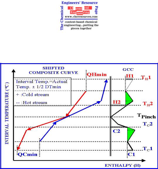
scale based upon process temperature having an allowance for temperature approach (DTmin). The Grand Composite Curve is then constructed from the enthalpy (horizontal) differences between the shifted composite curves at different temperatures. On the GCC, the horizontal distance separating the curve from the vertical axis at the top of the temperature scale shows the overall hot utility consumption of the process.
Figure 7: Grand Composite Curve
Figure 7 shows that it is not necessary to supply the hot utility at the top temperature level. The
GCC indicates that we can supply the hot utility over two temperature levels T 1 (HP steam)
H
and TH2 (LP steam). Recall that, when placing utilities in the GCC, intervals, and not actual utility temperatures, should be used. The total minimum hot utility requirement remains the same: QHmin = H1 (HP steam) + H2 (LP steam). Similarly, QCmin = C1 (Refrigerant) +C2 (CW). The points TH2 and TC2 where the H2 and C2 levels touch the grand composite curve are called the “Utility Pinches.” The shaded green pockets represent the process-to-process heat exchange.
In summary, the grand composite curve is one of the most basic tools used in pinch analysis for the selection of the appropriate utility levels and for targeting of a given set of multiple utility levels. The targeting involves setting appropriate loads for the various utility levels by maximizing the least expensive utility loads and minimizing the loads on the most expensive utilities.
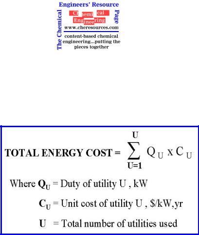
5. Estimation of Minimum Energy Cost Targets
Once the DTmin is chosen, minimum hot and cold utility requirements can be evaluated from the composite curves. The GCC provides information regarding the utility levels selected to meet QHmin and QCmin requirements.
If the unit cost of each utility is known, the total energy cost can be calculated using the energy equation given below.
6. Estimation of Heat Exchanger Network ( HEN ) Capital Cost Targets
The capital cost of a heat exchanger network is dependent upon three factors:
1.the number of exchangers,
2.the overall network area,
3.the distribution of area between the exchangers
Pinch analysis enables targets for the overall heat transfer area and minimum number of units of a heat exchanger network (HEN) to be predicted prior to detailed design. It is assumed that the area is evenly distributed between the units. The area distribution cannot be predicted ahead of design.
∙AREA TARGETING: The calculation of surface area for a single counter-current heat
exchanger requires the knowledge of the temperatures of streams in and out ( TLM i.e. Log Mean Temperature Difference or LMTD), overall heat transfer coefficient (U-value), and total heat transferred (Q). The area is given by the relation
Area = Q / [ U x TLM ]
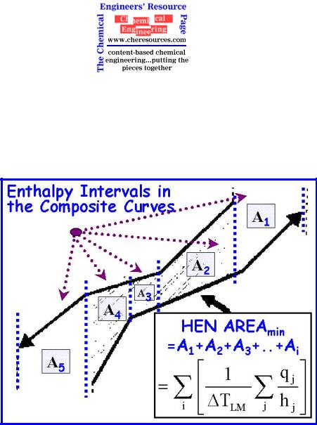
The composite curves can be divided into a set of adjoining enthalpy intervals such that within each interval, the hot and cold composite curves do not change slope. Here the heat exchange is assumed to be "vertical" (pure counter-current heat exchange). The hot streams in any enthalpy interval, at any point, exchanges heat with the cold streams at the temperature vertically below it. The total area of the HEN (Amin) is given by the formula in Figure 8, where i denotes the ith enthalpy and interval j denotes the jth stream and TLM denotes LMTD in the ith interval.
Figure 8: HEN AREA min Estimation from Composite Curves
The actual HEN total area required is generally within 10% of the area target as calculated above. With inclusion of temperature correction factors area targeting can be extended to non counter-current heat exchange as well.
∙NUMBER OF UNITS TARGETING: For the minimum number of heat exchanger units (Nmin) required for MER (minimum energy requirement or maximum energy recovery), the HEN can be evaluated prior to HEN design by using a simplified form of Euler’s graph theorem. In designing for the minimum energy requirement (MER), no heat transfer is allowed across the pinch and so a realistic target for the minimum number of units (NminMER) is the sum of the targets evaluated both above and below the pinch separately.
NminMER=[Nh+Nc+Nu–1]AP +[Nh+Nc+Nu–1]BP
Where : Nh = Number of hot streams
Nc = Number of cold streams
Nu = Number of utility streams
AP / BP : Above / Below Pinch
∙HEN TOTAL CAPITAL COST TARGETING: The targets for the minimum surface area (Amin) and the number of units (Nmin) can be combined together with the heat exchanger cost law to determine the targets for HEN capital cost (CHEN). The capital cost is annualized using an annualization factor that takes into account interest payments on borrowed capital. The equation used for calculating the total capital cost and exchanger cost law is given below.
For the Exchanger Cost Equation shown above, typical values for a carbon steel shell and tube exchnager would be a = 16,000, b = 3,200, and c = 0.7. The installed cost can be considered to be 3.5 times the purchased cost given by the Exchanger Cost Equation.
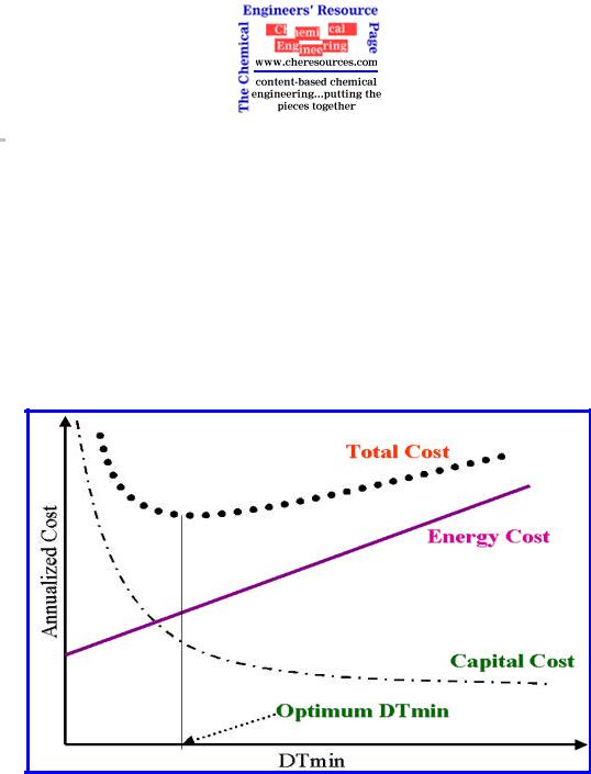
7. Estimation of Optimum DTmin Value by Energy-Capital Trade Off
To arrive at an optimum DTmin value, the total annual cost (the sum of total annual energy and capital cost) is plotted at varying DTmin values (Figure 7). Three key observations can be made from Figure 9:
a.An increase in DTmin values result in higher energy costs and lower capital costs.
b.A decrease in DTmin values result in lower energy costs and higher capital costs.
c.An optimum DTmin exists where the total annual cost of energy and capital costs is minimized.
Thus, by systematically varying the temperature approach we can determine the optimum heat recovery level or the DTminOPTIMUM for the process.
Figure 9: Energy-Capital Cost Trade Off (Optimum DTmin)
8. Estimation of Practical Targets for HEN Design
The heat exchanger network designed on the basis of the estimated optimum DTmin value is not always the most appropriate design. A very small DTmin value, perhaps 8 0C, can lead to a very complicated network design with a large total area due to low driving forces. The designer, in practice, selects a higher value (15 0C) and calculates the marginal increases in utility duties and area requirements. If the marginal cost increase is small, the higher value of

DTmin is selected as the practical pinch point for the HEN design.
Recognizing the significance of the pinch temperature allows energy targets to be realized by design of appropriate heat recovery network.
So what is the significance of the pinch temperature?
The pinch divides the process into two separate systems each of which is in enthalpy balance with the utility. The pinch point is unique for each process. Above the pinch, only the hot utility is required. Below the pinch, only the cold utility is required. Hence, for an optimum design, no heat should be transferred across the pinch. This is known as the key concept in Pinch Technology.
To summarize, Pinch Technology gives three rules that form the basis for practical network design:
∙No external heating below the Pinch.
∙No external cooling above the Pinch.
∙No heat transfer across the Pinch.
Violation of any of the above rules results in higher energy requirements than the minimum requirements theoretically possible.
Plus/Minus Principle: The overall energy needs of a process can be further reduced by introducing process changes (changes in the process heat and material balance). There are several parameters that could be changed such as reactor conversions, distillation column operating pressures and reflux ratios, feed vaporization pressures, or pump-around flow rates. The number of possible process changes is nearly infinite. By applying the pinch rules as discussed above, it is possible to identify changes in the appropriate process parameter that will have a favorable impact on energy consumption. This is called the "Plus/Minus Principle."
Applying the pinch rules to study of composite curves provide us the following guidelines:
∙Increase (+) in hot stream duty above the pinch.
∙Decrease (-) in cold stream duty above the pinch. This will result in a reduced hot utility target, and any
∙Decrease (-) in hot stream duty below the pinch.
∙Increase (+) in cold stream duty below the pinch will result in a reduced cold utility target.

These simple guidelines provide a definite reference for the adjustment of single heat duties such as vaporization of a recycle, pump-around condensing duty, and others. Often it is possible to change temperatures rather than the heat duties. The target should be to
∙Shift hot streams from below the pinch to above and
∙Shift cold streams from above the pinch to below.
The process changes that can help achieve such stream shifts essentially involve changes in following operating parameters:
∙reactor pressure/temperatures
∙distillation column temperatures, reflux ratios, feed conditions, pump around conditions, intermediate condensers
∙evaporator pressures
∙storage vessel temperatures
For example, if the pressure for a feed vaporizer is lowered, vaporization duty can shift from above to below the pinch. The leads to reduction in both hot and cold utilities.
Appropriate Placement Principles: Apart from the changes in process parameters, proper integration of key equipment in process with respect to the pinch point should also be considered. The pinch concept of “Appropriate Placement” (integration of operations in such a way that there is reduction in the utility requirement of the combined system) is used for this purpose. Appropriate placement principles have been developed for distillation columns, evaporators, heat engines, furnaces, and heat pumps. For example, a single-effect evaporator having equal vaporization and condensation loads, should be placed such that both loads balance each other and the evaporator can be operated without any utility costs. This means that appropriate placement of the evaporator is on either side of the pinch and not across the pinch.
In addition to the above pinch rules and principles, a large number of factors must also be considered during the design of heat recovery networks. The most important are operating cost, capital cost, safety, operability, future requirements, and plant operating integrity. Operating costs are dependent on hot and cold utility requirements as well as pumping and compressor costs. The capital cost of a network is dependent on a number of factors including the number of heat exchangers, heat transfer areas, materials of construction, piping, and the cost of supporting foundations and structures.
With a little practice, the above principles enable the designer to quickly pan through 40-50 possible modifications and choose 3 or 4 that will lead to the best overall cost effects.
The essence of the pinch approach is to explore the options of modifying the core process design, heat exchangers, and utility systems with the ultimate goal of reducing the energy and/or capital cost.
9. Design of Heat Exchanger Network
The design of a new HEN is best executed using the "Pinch Design Method (PDM)". The systematic application of the PDM allows the design of a good network that achieves the energy targets within practical limits. The method incorporates two fundamentally important features: (1) it recognizes that the pinch region is the most constrained part of the problem (consequently it starts the design at the pinch and develops by moving away) and (2) it allows the designer to choose between match options.
In effect, the design of network examines which "hot" streams can be matched to "cold" streams via heat recovery. This can be achieved by employing “tick off” heuristics to identify the heat loads on the pinch exchanger. Every match brings one stream to it target temperature. As the pinch divides the heat exchange system into two thermally independent regions, HENs for both above and below pinch regions are designed separately. When the heat recovery is maximized the remaining thermal needs must be supplied by hot utility.
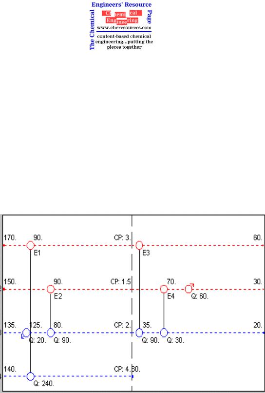
The graphical method of representing flow streams and heat recovery matches is called a
‘grid diagram’ (Figure 10).
Figure 10: Typical Grid Diagram
All the cold (blue lines) and hot (red line) streams are represented by horizontal lines. The entrance and exit temperatures are shown at either end. The vertical line in the middle represents the pinch temperature. The circles represent heat exchangers. Unconnected circles

represent exchangers using utility heating and cooling.
The design of a network is based on certain guidelines like the “CP Inequality Rule”, "Stream Splitting”, "Driving Force Plot" and "Remaining Problem Analysis". The stepwise procedure can be understood better with the help of an example problem (Link-5).
Having made all the possible matches, the two designs above and below the pinch are then brought together and usually refined to further minimize the capital cost. After the network has been designed according to the pinch rules, it can be further subjected to energy optimization. Optimizing the network involves both topological and parametric changes of the initial design in order to minimize the total cost. For more details on HEN Design check the Link –6 at the end of the article.