REGR_ (Linear Regression) Functions

REFTOHEX(BUILDING)

--------------------------------------------------------------------------

0000220208859B5E9255C31760E034080020825436859B5E9255C21760E034080020825436

REGR_ (Linear Regression) Functions

The linear regression functions are:

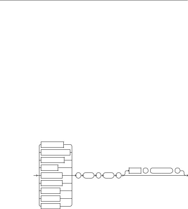
Syntax linear_regr::=

REGR_SLOPE

REGR_INTERCEPT

REGR_COUNT

REGR_R2

OVER ( analytic_clause )

REGR_AVGY

REGR_SXX

REGR_SYY

REGR_SXY

Functions 6-129

REGR_ (Linear Regression) Functions

See Also: "Analytic Functions" on page 6-10 for information on syntax, semantics, and restrictions

Purpose

The linear regression functions fit an ordinary-least-squares regression line to a set of number pairs. You can use them as both aggregate and analytic functions.

See Also:

Oracle applies the function to the set of (expr1, expr2) pairs after eliminating all pairs for which either expr1 or expr2 is null. Oracle computes all the regression functions simultaneously during a single pass through the data.

expr1 is interpreted as a value of the dependent variable (a "y value"), and expr2 is interpreted as a value of the independent variable (an "x value"). Both expressions must be numbers.

■REGR_SLOPE returns the slope of the line. The return value is a number and can be null. After the elimination of null (expr1, expr2) pairs, it makes the following computation:

COVAR_POP(expr1, expr2) / VAR_POP(expr2)

■REGR_INTERCEPT returns the y-intercept of the regression line. The return value is a number and can be null. After the elimination of null (expr1, expr2) pairs, it makes the following computation:

AVG(expr1) - REGR_SLOPE(expr1, expr2) * AVG(expr2)

■REGR_COUNT returns an integer that is the number of non-null number pairs used to fit the regression line.

■REGR_R2 returns the coefficient of determination (also called "R-squared" or "goodness of fit") for the regression. The return value is a number and can be null. VAR_POP(expr1) and VAR_POP(expr2) are evaluated after the elimination of null pairs. The return values are:

6-130 Oracle9i SQL Reference

REGR_ (Linear Regression) Functions

NULL if VAR_POP(expr2) = 0

1 if VAR_POP(expr1) = 0 and VAR_POP(expr2) != 0

POWER(CORR(expr1,expr),2) if VAR_POP(expr1) > 0 and VAR_POP(expr2 != 0

All of the remaining regression functions return a number and can be null:

■REGR_AVGX evaluates the average of the independent variable (expr2) of the regression line. It makes the following computation after the elimination of null (expr1, expr2) pairs:

AVG(expr2)

■REGR_AVGY evaluates the average of the dependent variable (expr1) of the regression line. It makes the following computation after the elimination of null (expr1, expr2) pairs:

AVG(expr1)

REGR_SXY, REGR_SXX, REGR_SYY are auxiliary functions that are used to compute various diagnostic statistics.

■REGR_SXX makes the following computation after the elimination of null (expr1, expr2) pairs:

REGR_COUNT(expr1, expr2) * VAR_POP(expr2)

■REGR_SYY makes the following computation after the elimination of null (expr1, expr2) pairs:

REGR_COUNT(expr1, expr2) * VAR_POP(expr1)

■REGR_SXY makes the following computation after the elimination of null (expr1, expr2) pairs:

REGR_COUNT(expr1, expr2) * COVAR_POP(expr1, expr2)

The following examples are based on the sample tables sh.sales and sh.products.

General Linear Regression Example

The following example provides a comparison of the various linear regression functions:

Functions 6-131

REGR_ (Linear Regression) Functions

REGR_SLOPE and REGR_INTERCEPT Examples

The following example determines the slope and intercept of the regression line for the amount of sales and sale profits for each fiscal year:

SELECT t.fiscal_year,

REGR_SLOPE(s.amount_sold, s.quantity_sold) "Slope", REGR_INTERCEPT(s.amount_sold, s.quantity_sold) "Intercept"

The following example determines the cumulative slope and cumulative intercept of the regression line for the amount of and quantity of sales for two products (270 and 260) for weekend transactions (day_number_in_week = 6 or 7) during the last three weeks (fiscal_week_number of 50, 51, or 52) of 1998:

6-132 Oracle9i SQL Reference

REGR_ (Linear Regression) Functions

SELECT t.fiscal_month_number "Month", t.day_number_in_month "Day", REGR_SLOPE(s.amount_sold, s.quantity_sold)

OVER (ORDER BY t.fiscal_month_desc, t.day_number_in_month) AS CUM_SLOPE, REGR_INTERCEPT(s.amount_sold, s.quantity_sold)

OVER (ORDER BY t.fiscal_month_desc, t.day_number_in_month) AS CUM_ICPT FROM sales s, times t

WHERE s.time_id = t.time_id AND s.prod_id IN (270, 260) AND t.fiscal_year=1998

AND t.fiscal_week_number IN (50, 51, 52) AND t.day_number_in_week IN (6,7)

ORDER BY t.fiscal_month_desc, t.day_number_in_month;

REGR_COUNT Examples

The following example returns the number of customers in the customers table (out of a total of 319) who have account managers.

SELECT REGR_COUNT(customer_id, account_mgr_id) FROM customers;

REGR_COUNT(CUSTOMER_ID,ACCOUNT_MGR_ID)

--------------------------------------

231

The following example computes the cumulative number of transactions for each day in April of 1998:

SELECT UNIQUE t.day_number_in_month,

REGR_COUNT(s.amount_sold, s.quantity_sold)

Functions 6-133

REGR_ (Linear Regression) Functions

OVER (PARTITION BY t.fiscal_month_number

ORDER BY t.day_number_in_month) "Regr_Count"

FROM sales s, times t

WHERE s.time_id = t.time_id

REGR_R2 Examples

The following example computes the coefficient of determination of the regression line for amount of sales greater than 5000 and quantity sold:

SELECT REGR_R2(amount_sold, quantity_sold) FROM sales WHERE amount_sold > 5000;

REGR_R2(AMOUNT_SOLD,QUANTITY_SOLD)

----------------------------------

.024087453

The following example computes the cumulative coefficient of determination of the regression line for monthly sales amounts and quantities for each month during 1998:

SELECT t.fiscal_month_number, REGR_R2(SUM(s.amount_sold), SUM(s.quantity_sold)) OVER (ORDER BY t.fiscal_month_number) "Regr_R2"

FROM sales s, times t WHERE s.time_id = t.time_id AND t.fiscal_year = 1998

GROUP BY t.fiscal_month_number ORDER BY t.fiscal_month_number;

FISCAL_MONTH_NUMBER Regr_R2

------------------- ----------

1

2 1

6-134 Oracle9i SQL Reference

REGR_ (Linear Regression) Functions

3.927372984

4.807019972

5.932745567

6.94682861

7.965342011

8.955768075

9.959542618

10.938618575

11.880931415

12.882769189

REGR_AVGY and REGR_AVGX Examples

The following example calculates the regression average for the amount and quantity of sales for each year:

SELECT t.fiscal_year,

REGR_AVGY(s.amount_sold, s.quantity_sold) "Regr_AvgY", REGR_AVGX(s.amount_sold, s.quantity_sold) "Regr_AvgX"

FROM sales s, times t WHERE s.time_id = t.time_id GROUP BY t.fiscal_year;

FISCAL_YEAR Regr_AvgY Regr_AvgX

----------- ---------- ----------

1998 716.602044 13.0584283

1999 714.910831 13.0665536

2000 717.331304 13.0479781

The following example calculates the cumulative averages for the amount and quantity of sales profits for product 260 during the last two weeks of December 1998:

SELECT t.day_number_in_month, REGR_AVGY(s.amount_sold, s.quantity_sold)

OVER (ORDER BY t.fiscal_month_desc, t.day_number_in_month) "Regr_AvgY",

REGR_AVGX(s.amount_sold, s.quantity_sold)

OVER (ORDER BY t.fiscal_month_desc, t.day_number_in_month) "Regr_AvgX"

FROM sales s, times t WHERE s.time_id = t.time_id

AND s.prod_id = 260

AND t.fiscal_month_desc = ’1998-12’ AND t.fiscal_week_number IN (51, 52)

ORDER BY t.day_number_in_month;

Functions 6-135

REGR_ (Linear Regression) Functions

REGR_SXY, REGR_SXX, and REGR_SYY Examples

The following example computes the REGR_SXY, REGR_SXX, and REGR_SYY values for the regression analysis of amount and quantity of sales for each year in the sample sh.sales table:

SELECT t.fiscal_year,

REGR_SXY(s.amount_sold, s.quantity_sold) "Regr_sxy", REGR_SYY(s.amount_sold, s.quantity_sold) "Regr_syy", REGR_SXX(s.amount_sold, s.quantity_sold) "Regr_sxx"

FROM sales s, times t WHERE s.time_id = t.time_id GROUP BY t.fiscal_year;

FISCAL_YEAR Regr_sxy Regr_syy Regr_sxx

----------- ---------- ---------- ----------

1998 1620591607 2.3328E+11 32809865.2

1999 1955866724 2.7695E+11 39637097.2

2000 2127877398 3.0630E+11 43226509.7

The following example computes the cumulative REGR_SXY, REGR_SXX, and REGR_SYY statistics for amount and quantity of weekend sales for products 270 and 260 for each year-month value in 1998:

SELECT t.day_number_in_month, REGR_SXY(s.amount_sold, s.quantity_sold)

OVER (ORDER BY t.fiscal_year, t.fiscal_month_desc) "Regr_sxy",

6-136 Oracle9i SQL Reference