analog_system_lab_pro_manual

DIODE

1N4448 Small Signal Diode

appendix B

Simulation models are very useful in the design phase of an electronic system. Before a system is actually built using real components, it is necessary to perform a ‘software breadboarding’ exercise through simulation to verify the functionality of the system and to measure its performance. If the system consists of several building blocks B1, B2, ..., Bn, the simulator requires a mathematical representation of each of these building blocks in order to predict the system performance. Let us consideraverysimpleexampleofapassivecomponentsuchasaresistor.Ohm’slaw can be used to model the resistor if we intend to use the resistor in a DC circuit. But if the resistor is used in a high frequency application, we may have to think about the parasitic inductances and capacitances associated with the resistor. Similarly, the voltage and current may not have a strict linear relation due to the dependence of the resistivity on temperature of operation, skin effect, and so on. This example illustrates that there is no single model for an electronic component. Depending on the application and the accuracy desired, we may have to use simpler or more complex mathematical models.

We will use another example to illustrate the above point. The MOS transistor, which is the building block of most integrated circuits today, is introduced at the beginning of the course on VLSI design. In a digital circuit, the transistor may be simply modeled as an ideal switch that can be turned on or off by controlling the gate voltage. This model is sufficient if we are only interested in understanding the functionality of the circuit. If we wish to analyze the speed of operation of the circuit or the power dissipation in the circuit, we will need to model the parasitics associated with the transistors. If the same transistor is used in an analog circuit, the model that we use in the analysis would depend on the accuracy which we want in the analysis. We may perform different kinds of analysis for an analog circuit -

DC analysis, transient analysis, and steady-state analysis. Simulators such as SPICE require the user to specify the model for the transistor. There are many different models available today for the MOS transistor, depending on the desired accuracy. The level-1 model captures the dependence of the drain-to-source current on the gate-to-source and drain-to-source voltages, the mobility of the majority carrier, the width and length of the channel, and the gate oxide thickness. It also considers non-idealities such as channel length modulation in the saturation region, and the dependence of the threshold voltage on the source-to-bulk voltage. More complex models for the transistor are available, which have more than 50 parameters.

B.1 Micromodels

If you have built an operational amplifier using transistors, a straight-forward way to analyze the performance of the OP-Amp is to come up with the micromodel of the OPAMAP, where each transistor is simply replaced with its corresponding simulation model. Micromodels will lead to accurate simulation, but will prove computationally

page 84

intensive. As the number of nodes in the circuit increases, the memory requirement will be higher and the convergence of the simulation can take longer.

A macromodel is a way to address the problem of space-time complexity mentioned above. In today’s electronic systems we make use of analog circuits such as operational amplifiers, data converters, PLL, VCO, voltage regulators, and so on.

The goal of the system designer is not only to get a functionally correct design, but also to optimize the cost and performance of the system. The system-level cost and performance depend on the way the building blocks B1, B2,..., Bn have been implemented. For example, if B1 is an OP-Amp, we may have several choices of operational amplifiers. Texas Instruments offers a large number of operational amplifiers that a system designer can choose from. Refer to Table B.1. As you will see, there are close to 2000 types of operational amplifiers available! These are categorized into 17 different bins to make the selection simpler. However, you will notice that 240 varieties are available in the category of Standard Linear amplifers! How does a system designer select from this large collection? To understand this, you must look at the characteristics of a standard linear amplifier - these include the number of operational amplifiers in a single package, the Gain Bandwidth Product of the amplifier, the CMRR, Vs (min), Vs (max), and so on. See http://tinyurl.com/ti-std-linear. The website allows you to specify these parameters and narrow your choices.

But how does one specify the parameters for the components? The overall system performance will depend on the way the parameters for the individual components have been selected. For example, the gain-bandwidth product of an operational amplifier B1 will influence a system-level parameter such as the noise immunity or stability. If one has n components in the system, and there are m choices for each component, there are m·n possible system configurations. Even if we are able to narrow the choices through some other considerations, we may still have to evaluate several system configurations. Performing simulations using micromodels will be a painstaking and non-productive way of selecting system configurations.

B.2 Macromodels

A macromodel is a mathematical convenience that helps to reduce simulation complexity. The idea is to replace the actual circuit by something that is simpler, but is nearly equivalent in terms of input characteristics, output characteristics, and feedforward characteristics. Simulation of a complete system becomes much more simple when we use macromodels for the blocks. Manufacturers of semiconductors provide macromodels for their products to help system designers in the process of system configuration selection. The macromodels can be loaded into a simulator.

Analog System Lab Kit PRO

Table B.1: Operational Amplifiers available from Texas Instruments

As you can guess, there is no single macromodel for an IC. A number of macromodels can be derived, based on the level of accuracy desired and the computational complexity that one can afford. A recommended design methodology is to start with a simple macromodel for the system components and simulate the system. A stepwise refinement procedure may be adopted and more accurate models can be used for selected components when the results are not satisfactory.

Analog System Lab Kit PRO

appendix B

page 85

appendix B

Notes on Appendix B:

appendix C

C.1 Introduction

In any analog lab, an oscilloscope is required to display waveforms at different points in the circuit under construction in order to verify circuit operation and, if necessary, redesign the circuit. High-end oscilloscopes are needed for measurements and characterization in labs. Today, solutions are available to students for converting a PC into an oscilloscope. These solutions require some additional hardware to route the analog signals to the PC for observation; they also require software that provides the graphical user interface to convert a PC display into an oscilloscope. Since most students have access to a PC or laptop today, we have designed the Analog System Lab such that a PC-based oscilloscope solution can be used along with ASLK PRO. We believe this will reduce the dependence of

the student on a full-edged lab. In this chapter, we will review a solution for a PC-based oscilloscope. The components on the ASLK PRO can be used to build the interface circuit needed to convert the PC into an oscilloscope.

One of the solutions for a “PC oscilloscope” is Zelscope

[33] which works on personal computers running Microsoft Windows XP. The hardware requirements for the PC are modest (300+ MHz clock, 64+ MB memory). It uses the sound card in the PC for converting the analogsignalsintodigitalform.TheZelscopesoftware, which requires about 1 MB space, is capable of using the digitized signal to display waveforms as well as the frequency spectrum of the analog signal. At the

‘line in’ jack of the sound card, the typical voltage

should be about 1 volt AC; hence it is essential to protect the sound card from over voltages. A buffer amplifier circuit is required to protect the sound card from overvoltages. Two copies of such a circuit are needed to implement a dual-channel oscilloscope. The buffer amplifier circuit is shown in Figure C.1 and has been borrowed from [32].

Limitations

•Not possible to display DC voltages (due to input capacitor of sound card blocks DC)

•Low frequency range (10 Hz-20 kHz)

•Measurement is not very accurate

Figure C.1:

Buffer circuit needed to interface an Analog Signal to Oscilloscope

page 88

Analog System Lab Kit PRO

appendix D

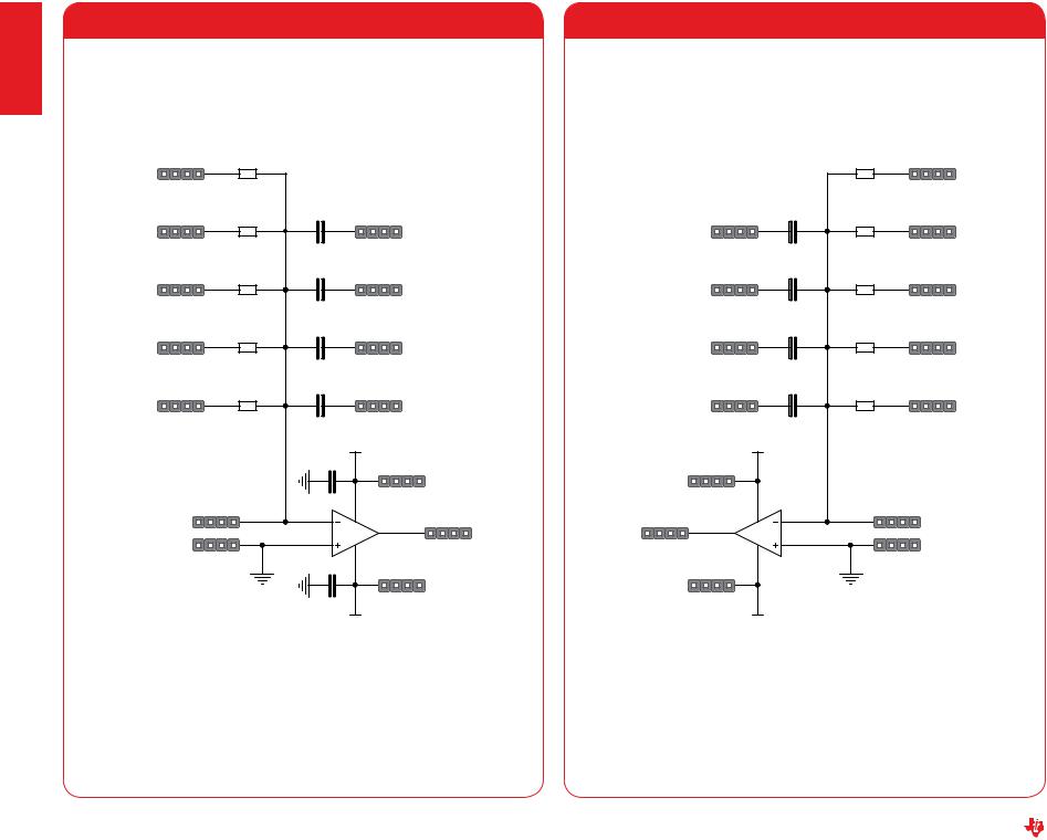
OP AMP TYPE I - A - INVERTING

OP AMP TYPE I - B - INVERTING

HD181

-10V

VCC-10