Analysis

Angular width

The Polar Iso-Candela plot is displayed over a subset of a hemisphere of the entered angular width. The angle is entered in degrees.

Set Max/Min

Sets the Max or Min value to plot. If the item is enabled, the value entered in the edit box will be used when the plot is updated.

Log Plot

Checking this box displays the data on a logarithmic scale. This is especially useful when you need to see details in the very lowest data values. This might be needed, for example, in a stray light analysis.

Color Map

Use this drop-down list to choose either grayscale or one of several color-coded schemes. The choice of color affects both the display and the contour map display on the Iso-Candela Plot as well as the distribution plots.

Auto levels

The Auto levels check box controls the contour levels in the Polar Iso-Candela plot. If the Auto levels box is checked, TracePro divides the display of intensity values evenly into the number of levels defined in the Number entry in the Levels part of the dialog box. When you click the Apply button, the plot is updated with the new levels.

Selection

If Auto levels is not checked, TracePro uses the levels defined in the list box on the right hand side of the Levels section of the dialog box. You can customize the levels by moving numbers in and out of the box. Move numbers from the Selection box into the list by clicking the --> button, and out (to remove them from the list) by clicking the <-- button.

You can use Auto levels for a desired number of contours and TracePro will equally space the number over the flux or candela range plotted.

Number

This entry controls the number of Auto levels displayed either in the color-coded intensity or contour Polar Iso-Candela plot.

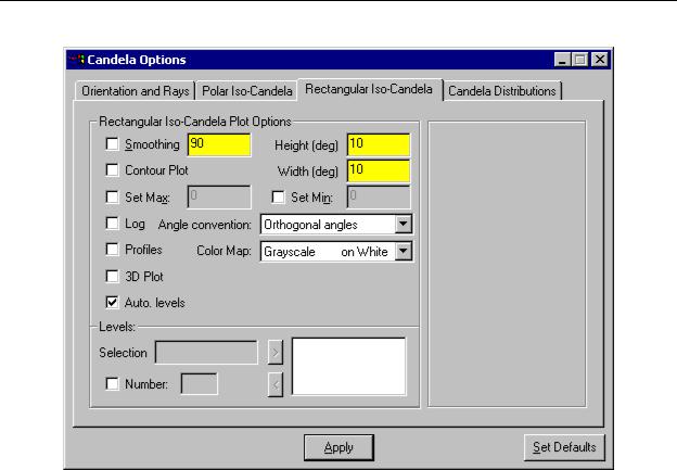
Rectangular Iso-Candela

A Rectangular Plot shows the intensity or candela distribution as a function of vertical and horizontal angles. This is in contrast to the Polar Plot, in which the pole of the polar coordinates is in the center of the plot. For the Rectangular Plot, the equator is in the center of the plot, so that the angles are vertical and horizontal angles. A square angular region is displayed on the plot. The size of the region can be controlled in this area of the dialog box.

Analysis Menu

FIGURE 6.15 - Candela Options dialog with the Rectangular Iso-Candela tab displayed.

Height and Width

These entries control the size of the angular region that is plotted. The dimensions are in degrees. The center of the plot is along the direction of the Normal Vector. The top of the plot is along the direction of the Up Vector.

Angle Convention

The Angle convention defines the method used to display the rectangular plot. Selecting Orthogonal angles displays the angular data projected onto the x-z and y-z orthogonal planes. Type A and Type B goniometers use the angle conventions outlined in the Lighting Handbook, published by the Illuminating Engineering Society of North America (IESNA).

Profiles

Display an XY plot in the same window with data slices based on the mouse cursor position.

3D Plot

This option produces a 3D relief plot using OpenGL.

Analysis

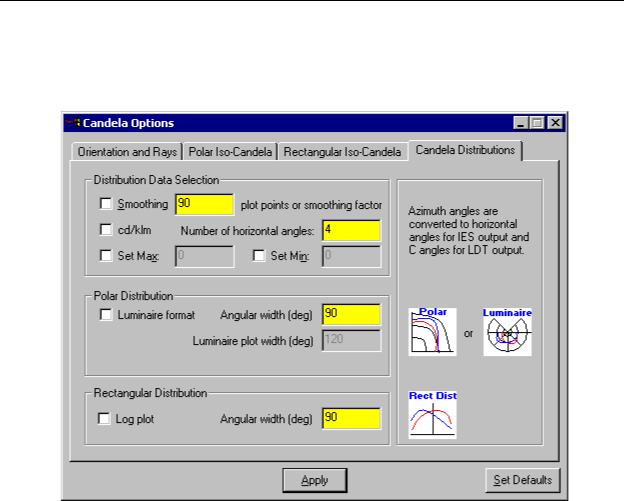
Candela Distributions

The Candela Distribution plots are defined as slices of the sphere containing the emitting source. The number of slices and resolution can be defined by the user.

FIGURE 6.16 - Candela Options dialog with the Candela Distributions tab displayed.

Smoothing

This option determines whether smoothing is performed on the data slices. If enabled, the number in the smoothing box is used as a smoothing factor. If smoothing is off, the number sets the number of points about the slices to display in the plot.

cd/Klm

Scales output to cd per 1000 lumens. This is a common scale factor for lighting output.

Number of horizontal angles

Sets the number of horizontal angles to plot. The value set here corresponds to the horizontal angles in IES (IESNA) format and to C angles in ldt (eulumdat) format files. See “IESNA and Eulumdat formats” on page 6.25.

Analysis Menu

Luminaire format

When checked, the format of the Polar Candela Distribution plot changes to conform to the standard Luminaire Design format, with the Normal Vector pointing down.

Angular width

Sets the angular width of the luminaire display in degrees. The width for polar and rectangular distributions can be set individually.

Luminaire width

Sets the angular range of the display in degrees when the Luminaire format is selected.

Set Max/Min

Sets the Max or Min value to plot. If the item is enabled, the value entered in the edit box will be used when the plot is updated.

Log Plot

Checking this box displays the data on a logarithmic scale. This is especially useful when you need to see details in the very lowest data values. This might be needed, for example, in a stray light analysis.

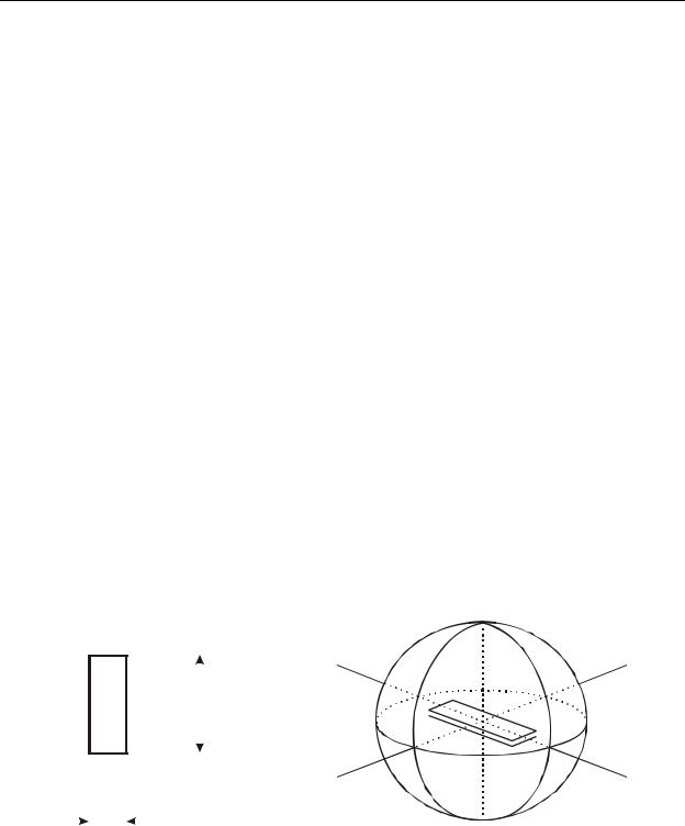
IESNA and Eulumdat formats

Data can be saved to a text file in IESNA (ies) and Eulumdat (ldt) formats. When saving the data to a text file via File|Save As or right clicking in the display window and selecting Save As..., the file format is selected with the file extension drop down box. The IES format is specified in IESNA (Illuminating Engineering Society of North America) standard LM-63-95. Figure 6.17 summarizes the IESNA conventions for angles used in the IESNA format.

FIGURE 6.17 - Conventions for vertical and horizontal angles used in standard IESNA format; (a) plan view of luminaire showing length and width in relation to horizontal angles, and (b) schematic showing

vertical and horizontal angles.1

Analysis

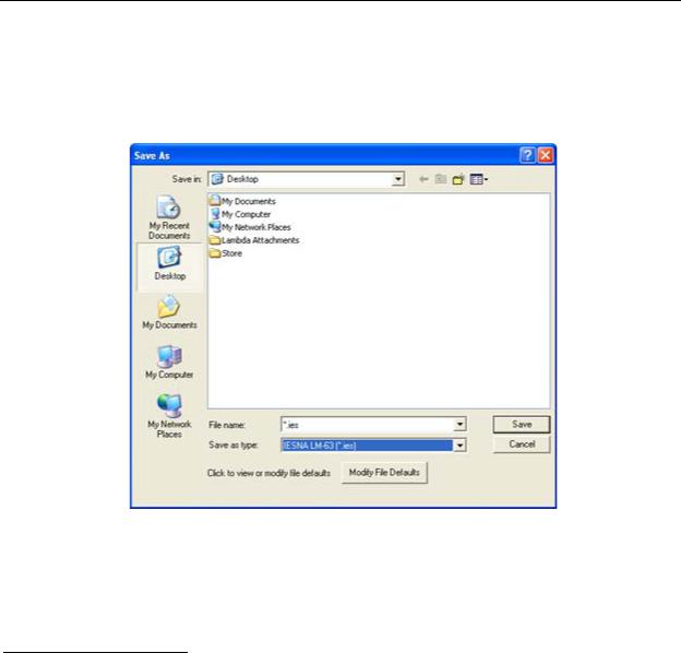
shows the dialog that appears when you select Save As. There are four options for the file types: text (*.txt), IESNA (*.ies), Eulumdat (*.ldt), and bitmap (*.bmp). The text file option saves the data to a text file. The bitmap option saves a bitmap figure of the plot. The IESNA and Eulumdat options provide a number of options to save the data. The following paragraphs explain and show these options.

FIGURE 6.18 - Save As dialog for candela plots.

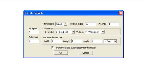
When the IESNA format is chosen in the File|Save As dialog, you are allowed to enter a number of inputs appropriate to the IESNA standard, including the number of lamps, symmetry and luminous dimensions (see Figure 6.19). This additional dialog is displayed upon selecting the *.ies option.

1.Reproduced from IESNA Standard File Format for Electronic transfer of Photometric Data, p.4, Illuminating Engineering Society of North America.

Analysis Menu

FIGURE 6.19 - The additional Save As dialog for the IESNA format allows you to enter a number of IESNA specific parameters.

The various options are (the bolded items denote the default values):

•Photometric measurement (i.e., type of goniometer): Type C, Type B, or Type A,

•Vertical angles: the number of angles to save in the vertical direction, 19,

•# Lamps: the number of lamps that provide the distibution to be saved, 1,

•Multiplier: the multiplier that should be applied to the data, 1,

•Symmetry, Horizontal (see Figure 6.17): the horizontal symmetry of the system, 0-0 degrees, 0-90 degrees, 0-180 degrees, or 0-360 degrees,

•Symmetry, Vertical (see Figure 6.17): the vertical symmetry of the system, 0-0 degrees, 0-180 degrees, or 90-180 degrees,

•# decimals: the number of decimals that will be saved for each number in the saved file, 6,

•Width: the width of the luminious area of the source in the designated units, 0,

•Length: the length of the of the luminious area of the source in the designated units, 0,

•Height: the height of the luminious area of the source in the designated units,

0,

•Combo box: units for the luminous dimensions of the source, in Feet or in Meters, and

•Checkbox: checking this box will open this dialog whenever the IESNA (*.ies) file type is selected. If the box is unchecked, then this dialog will not automatically open, but it can be manually opened by clicking on the Modify File Defaults button as shown in Figure 6.18.

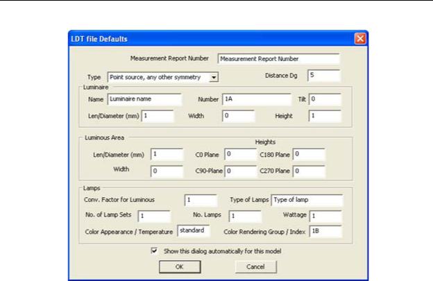
When the Eulumdat format is chosen in the File|Save As dialog, you are allowed to enter a number of inputs appropriate to the Eulumdat standard, including the number of lamps, symmetry and luminous dimensions (see Figure 6.20). This additional dialog is displayed upon selecting the *.ldt option.

Analysis

FIGURE 6.20 - The additional Save As dialog for the Eulumdat format allows you to enter a number of Eulumdat specific parameters.

The various options are (the bolded items denote the default values):

•Measurement Report Number: the designator given to the report for this file save, Measurement Report Number,

•Type: the type of source and its symmetry, point source, vertical axis symmetry; linear luminaire; or point source, any other symmetry (note that only the linear luminaire option is subdivided into longitudinal and transverse directions),

•Distance Dg: the distance in degrees between luminous intensities in the C- plane, 5,

•Luminaire Name: name of the luminaire, Luminaire name,

•Luminaire Number: the luminaire number for quality control, 1,

•Luminaire Tilt: the tilt angle of the luminaire during testing, 0,

•Luminaire Len/Diameter: the length or diameter of the luminaire in mm, 1,

•Luminaire Width: the width of the luminaire in mm, with 0 for circular luminaires, 0,

•Luminaire Height: the height of the luminaire in mm, 1,

•Luminous Area Len/Diameter: the length or diameter of the luminous area in mm, 1,

•Luminious Area Width:the width of the luminous area in mm, 0,

•C0 Plane: the height of the luminous are C0-Plane in mm, 0,

•C90 Plane: the height of the luminous are C90-Plane in mm, 0,