Ray Tracing

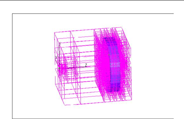
FIGURE 5.27 - Octree Voxels for a simple telescope.

Raytrace Type

The default raytrace type is Exact Raytracing which represents spline surfaces to the limit of numeric precision during the raytrace. However if you wish to speed up the raytrace at the expense of accuracy, you can choose Faceted Splines which represents NURBS or spline surfaces by triangular plane facets during the raytrace. Intersecting a ray with a spline surface is time-consuming, so you may see a significant speedup in the ray-trace by representing splines by facets. The Normal Tolerance controls the angle between the actual surface normal and the facet surface normal. TracePro creates more facets until the largest angle difference for any facet is less than this tolerance. The default value is one degree, which is a good compromise between speed, memory consumption, and accuracy. The tighter the tolerance, the more facets are created, and the better the accuracy of the ray-trace, but the slower the speed. You will have to decide whether using facets for splines is appropriate for your model, and what balance between speed, memory consumption, and accuracy is best. In general, the tighter the normal tolerance, the more voxels you will need to maintain the speed of the ray-trace. When you select Faceted Splines, then, you should also select Fastest Raytrace or perhaps even a custom number of voxels when using Uniform Voxels, or a large tree depth when using Octree Voxels. Finally, remember that if you choose Faceted Splines, your ray-trace speed may improve by also selecting Octree voxels.

A hybrid solution can be set using the Accelerated Raytracing mode. This combines facets to find a close intersection with exact raytracing to locate the intersection of the surface.

Raytrace Options

Which surfaces are splines?

When you import a model from another CAD program, some of the surfaces may be NURBS or spline surfaces. If you expand each surface in the system tree, the type of surface is displayed. In general, any surface that is not a primitive surface type is a spline. The primitive surface types in TracePro are Plane, Sphere, Cone, and Torus. For example, if a surface was parabolic or elliptical in the CAD program, it will be exported as a spline. If a surface is created as a Parabolic Reflector in TracePro, it is represented as a paraboloid of revolution while in TracePro but will be exported as a spline. Therefore, a parabolic reflector that is created in TracePro will be ray-traced much faster than one created in a CAD program and imported into TracePro. You can regain some of this speed at the expense of accuracy by choosing the Faceted Splines setting. Finally, if you create, for example, a parabolic reflector in TracePro and alter it by a Boolean operation, it will become a spline. In this case the ray-trace speed will slow, and you can regain much of this speed by selecting Faceted Splines.

You may be able to convert some of the spline surfaces to primitive surfaces if they started as primitive surfaces but were changed to splines by the CAD program as it exported the file. This may happen depending on the originating CAD program and the settings that were in place when the file was exported. To convert the surfaces to primitives, use Tools|Healing|Autoheal or Tools|Healing|Heal|Simplify. See “Healing Imported Data” on page 2.38

Gradient Index Substep Tolerance Standard Expert

The Gradient Index Substep Tolerance lets you trade-off accuracy vs. speed while tracing rays through an object with a Gradient Index property on it. TracePro uses an adaptive stepping algorithm. Each substep takes a curved trajectory through the gradient index material. The length of the substep is a function of many variables including the gradient index profile in the local region of the material and the user-supplied substep tolerance. As the ray proceeds through the material, optical position and optical path errors are not permitted to exceed this tolerance. When this tolerance is met, a new substep is created. A smaller tolerance will improve accuracy at the expense of raytrace speed, while a larger tolerance will speed up the raytrace at the expense of accuracy. The optimal setting depends on the specific characteristics of your model. You should experiment with different settings for a particular model to determine the optimal setting.

Maximum Nested Objects

The Maximum nested objects setting specifies the number of levels of embedded objects that are allowed for a given raytrace.

The default value for Maximum Nested Objects is 10. In the event that a given model has more than 10 nested objects, rays intersecting with the 11th embedded object will be terminated, and a message will appear in the Message/Macro Window. Selecting a value greater than 10 allows these rays to continue.

Changing the Maximum Nested Objects selection from the default value has a negligible impact on raytrace times or RAM consumption. It is best to operate with the default selection, and manually increase it only in the case where error messages occur.