Ray Tracing

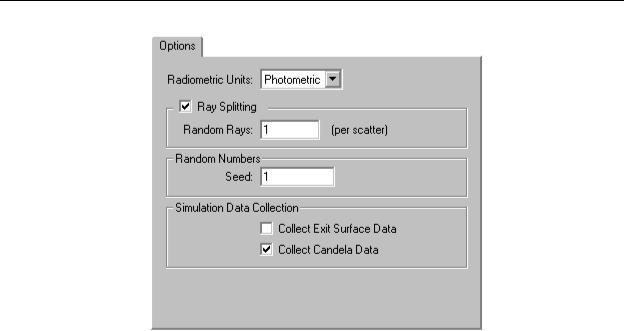
FIGURE 5.23 - Options Tab for TracePro LC

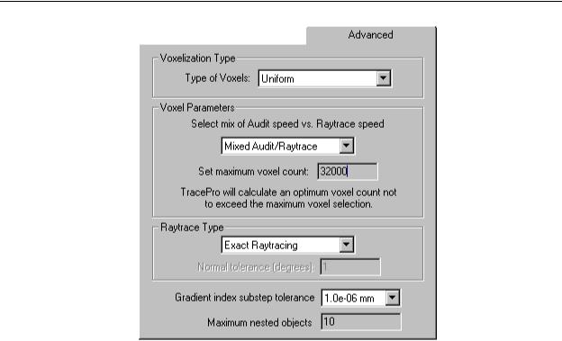
Advanced Options

The Advanced tab of the Raytrace Options dialog, as shown in Figure 5.24, provides controls to enhance ray-trace speed, change the precision for tracing rays in gradient index materials, and control the number of nested objects accommodated in TracePro. To control the ray-trace speed you can choose from two types of voxels. You also have the option to represent NURBS surfaces by facets.

Raytrace Options

FIGURE 5.24 - Advanced Tab (Uniform Options)

Voxelization Type

To speed up a ray-trace, TracePro uses object space partitioning to break up a model into small regions called voxels. Think of voxels as 3D pixels, including depth along with width and height. Using voxels involves a trade-off of ray-trace speed versus audit speed and memory consumption. For most analyses, you can leave this setting at Uniform. However, when you are using Raytrace Type: Faceted Splines you may see a significant improvement in ray-trace speed by choosing octree voxels. Some models with widely separated geometry may also see a speed improvement with octree voxels.

Voxel Parameters

The Voxel Parameters, in the center of the Advanced tab, change depending on whether you choose Uniform or Octree voxels.

Uniform voxels

Typically, you would start the analysis of a complex or large model by tracing rays at the Fastest Audit or Mixed Audit/Raytrace setting. Perform any system setup and determination of thresholds with a relatively small ray set. When you are ready to trace many rays, change to Fastest Raytrace. TracePro will calculate an optimal number of voxels to use, but no more than the number in Set maximum voxel count. If you feel that your model would benefit from more voxels than TracePro is choosing, select Maximize Voxel Count and set the Set maximum voxel count number to the number of voxels you desire. Be aware that more voxels use more memory. There is a minimum of 4 bytes of memory allocated for each voxel, and more memory is allocated for bigger models. At 4,000,000 voxels, you can expect a minimum of 16 MB of memory to be consumed. Figure 5.25

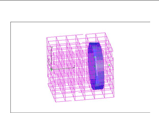
Ray Tracing

shows the voxels generated for a simple telescope using the Fastest Audit selection.

FIGURE 5.25 - Uniform Voxels for a simple telescope.

Octree voxels

If your model is very spread out with large regions of empty space, or if you are using Faceted Splines for Raytrace Type, you may see an increase in ray-trace speed by choosing octree voxels. Octree voxels are created recursively. TracePro starts with one voxel containing all the geometry in your model, then subdivides it into eight octants, or voxels, using three dividing planes. Each of these smaller voxels can be subdivided as well, and so on until criteria determined by the voxel parameters are met, creating a tree-like structure of voxels. Where there are more surfaces, edges, and facets, more subdividing will take place. This technique creates more voxels where they are needed, and fewer voxels where there is empty space. The Maximum Tree Depth determines the maximum number of times voxels can be subdivided. A usual number to use for this is in the range of

two to six. The maximum number of voxels created is on the order of 8N, where N is the maximum tree depth. For example, with N=2, no more than about 64 voxels will be created, while for N=6, no more than about 262,144 voxels will be created. Octree voxels use more memory per voxel than uniform voxels, with each voxel requiring at least 56 bytes, so with N=6, there may be 14MB or more of memory consumed. Also, empty octree voxels are slower to traverse than uniform voxels.

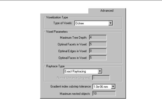
Raytrace Options

FIGURE 5.26 - Advanced Tab (Octree Options)

The Optimal settings are criteria for TracePro to create more voxels. TracePro will create more voxels during the audit until all of these criteria are met or until the

Maximum Tree Depth is reached. The Optimal Facets in Voxel is the target number of facets and applies only to faceted splines, when the Raytrace Type:Faceted Splines option is selected. The Optimal Edges in Voxel and the

Optimal Faces in Voxel settings apply only to non-faceted surfaces. In normal usage, you will not need to change these settings. Figure 5.27 shows Octree voxels generated for the simple telescope shown in Figure 5.25. The optical elements are widely spaced and you can see how few voxels are created between the elements while many are created close to surfaces and edges.