Applying Properties

sampling target for the diffracting aperture is applied to the surface that is defining the edge of the aperture.

How do I Set Up Diffraction?

Diffraction occurs in TracePro at a surface on which a diffraction property is defined. Setting up diffraction on a surface consists of four steps:

1.Select a surface on which you want to model diffraction. It can be the surface of a mirror or lens. If there is no surface where you want to model diffraction, you must define a “dummy object.” Locate the dummy object where you want the diffraction to occur, and select one surface of the object.

2.Place a check in the Aperture Diffraction check box located on the Diffraction tab of the Define|Apply Properties dialog box.

3.Set the Aperture Diffraction check box in the Raytrace Options dialog box found on the Analysis menu. This turns on diffraction for the current model.

4.Optionally, set the diffraction distance in the Raytrace Options dialog box. This information lets you limit model calculations to an area within a specified distance. The Aperture Diffraction distance is the maximum distance in millimeters from the diffraction edge at which the user wants the model rays to be calculated. Beyond that distance, it is assumed that rays proceed undeviated. If you’re not sure how to use this setting, leave it at its default value.

5.Add importance targets to the aperture surface. For more information about “Importance Sampling”, see page 4.22.

Using the Raytrace Flag

The raytrace flag property lets you exclude an object from a raytrace, which can speed up the raytrace. During the audit prior to the start of a raytrace, messages are displayed in the Macro/ Message Window to remind you which surfaces you have excluded from the raytrace.

To exclude an object from the raytrace, select the object. Open the Define|Apply Properties dialog box to select the Raytrace Flag tab. Mark the check-box on the Raytrace Flag tab dialog box. Click Apply.

Mueller Matrix Standard Expert

You can create and apply a polarizing element to a TracePro object by specifying its Mueller matrix. TracePro uses the Stokes vector-Mueller matrix method (Mueller calculus) for modeling polarized light.

Use the Define|Apply Properties dialog box and select Mueller matrix tab to apply polarization to a TracePro object. Use the Grid Raytrace dialog box also if you need to specify the polarization of the starting rays.

Mueller Matrix

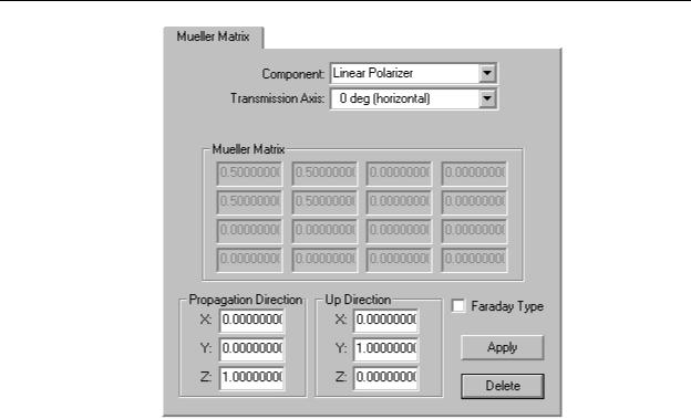
FIGURE 4.26 - The Apply Properties Dialog Box - Mueller Matrix tab

If you specify a Mueller matrix, you must also specify its orientation. Do this by specifying the “Up Direction” vector and the “Propagation Direction” vector at the bottom of the dialog box. Orientation vectors are specified in global coordinates. The direction vector specifies the direction in which light is traveling when the Mueller matrix has the specified effect.

TABLE 4.6. Mueller Matrix Options.

Component Selects one of several predefined types of polarizing components.

If you know the values of the Mueller Matrix or the component does not conform to one of the standard types select the Custom Component. The following options are displayed.

Applying Properties

TABLE 4.7. Options for Custom Mueller Matrix Data Entry.

When a ray traverses an object, the Stokes vector of the ray is transformed to the coordinate system of the Mueller matrix and then multiplied by the Mueller matrix to determine the new polarization state of the ray. Any flux that is absorbed by the Mueller matrix is recorded as the ray enters the object. That is, the incident flux on the surface as the ray leaves the object is lower in the amount absorbed by the Mueller matrix, similar to bulk absorption.

A Mueller matrix is a 4x4 matrix and a Stokes vector is a column vector of length 4. Therefore, multiplying a Stokes vector by a Mueller matrix produces a new Stokes vector. In this way a Stokes vector can be propagated through an optical system. For example, a Mueller matrix that does nothing is the unit matrix,

1 0 0 0

0 1 0 0 ,

0 0 1 0

0 0 0 1

while a horizontal polarizer is represented by

The Stokes vector for unpolarized light is

1

0 ,

0

0

while the Stokes vector for perfectly horizontally polarized light is

1

1 .

0

0

There is a collection of example Mueller matrices and Stokes vectors in the Technical Reference section. Discussions and examples of Mueller matrices and Stokes vectors can be found in many textbooks (for example, E.L. O’Neill, Introduction to Statistical Optics, Dover, ISBN: 0486673286 (1992); E. Collett,

Temperature

Polarized Light: Fundamentals and Applications, Dekker, ISBN: 0824787293 (1992); Shurcliff and Ballard, Polarized Light, van Nostrand (1964); Kliger, Lewis, and Randall, Polarized Light in Optics and Spectroscopy, Academic Press, ISBN: 0124149758 (1990)).

Mueller matrices must be defined with care – it is quite possible to create a Mueller matrix that is impossible, i.e. one that creates a resulting Stokes vector that is not physically possible.

Temperature Standard Expert

TracePro has a Surface and Object property for temperature. Material and Surface properties have data based on wavelength and temperature. During the raytrace audit the property data is updated to reflect the current surface and object temperatures. If an object has a defined temperature but the surfaces do not, the object temperature is applied to the surfaces. If no temperature is defined, the default value for the property is used.

As an example, consider a simple material property named “Temperature,” which has an index of 1.5 for 300K and 2.5 at 500K. The raytrace for the two cases is shown. The flux threshold has been set to 5% to eliminate most Fresnel reflections.

FIGURE 4.27 - Raytrace of block with example “Temperature” material applied, with n = 1.5 at T=300K

Applying Properties

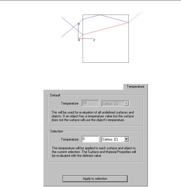
FIGURE 4.28 - Raytrace of block with example “Temperature” material applied, with n = 2.5 at T=500K

FIGURE 4.29 - Apply Properties Dialog Box, Temperature Tab

Temperature is applied like any other property, through the Apply Property dialog box. After selecting the objects and surfaces of the same temperature, enter the new temperature and press Apply to update the model.

Temperature is entered in units of degrees C, degrees F, or Kelvin.

Note: If a property is defined at only a single temperature, the surface and object temperatures are effectively ignored.

Note: The default temperature is not used in the current version of TracePro.